From DXF drawing to mesh

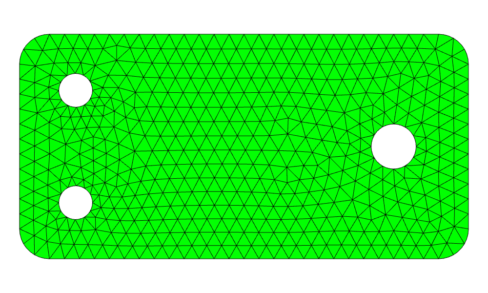
A part drawn in a CAD program reaches a finite-element mesh in three steps with planex2d. The drawing is read and its small gaps are closed, the boundaries that the simulation needs are named, and netgen meshes the face, with the edge names as its boundary names. The same steps start from an SVG drawing, a planar STEP or BREP file, a sketch from a .CATPart file, a circuit board or a Shapely polygon, each with its own reader. The first cell is the complete workflow, ready to copy and run, and the section Step by step runs it in parts, with the plots one looks at along the way.

The example is a mounting bracket of 120 × 60 mm with corners of radius 8, two bolt holes of diameter 9 and a pin hole of diameter 12. It is drawn in millimeters, with its outline, its holes and its center lines on three layers, in the file bracket.dxf. Its top edge stops 0.0002 mm short of the corner arc, as exported drawings often do.

import ngsolve as ngs
from ngsolve_webgpu.jupyter import Draw
import planex as px

bracket = px.Face(px.FromDXF("bracket.dxf", layers=["outline", "holes"], tol=1e-6))
bracket.name = "steel"
bracket.edges(name="holes").name = "bolts"
bracket.edges(name="bolts").Max("radius").name = "pin"

mesh = ngs.Mesh(px.OCCGeometry(bracket).GenerateMesh(maxh=0.004))
mesh.Curve(3)
print(mesh.ne, "elements |", mesh.GetMaterials(), "|", sorted(set(mesh.GetBoundaries())))
print("mesh area", ngs.Integrate(1, mesh), "| face area", bracket.mass)
Draw(mesh)

954 elements | ('steel',) | ['bolts', 'outline', 'pin']
mesh area 0.0069047246892775934 | face area 0.006904730091834054

▶ Click to interact

Step by step

Reading the drawing

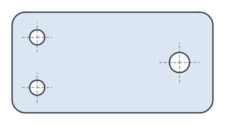
px.FromDXF reads the lines, arcs and circles of the drawing as exact edges, one wire per chain, and px.Face makes the face of them, with the holes found from how the loops nest (see Objects in planex2d). layers takes only the outline and the holes, so the center lines stay out of the part, and each edge keeps its layer as its name. The reader takes the unit from the drawing’s header, millimeters here, and returns meters, so the bracket is 0.12 long (see Units). tol joins ends that lie closer together than it, also in meters. It closes the gap at the top edge, which would otherwise leave the outline open, so that px.Face would refuse it (Figure 1). See Files for the readers of every format and their options.

import ngsolve as ngs
from ngsolve_webgpu.jupyter import Draw
import planex as px

bracket = px.Face(px.FromDXF("bracket.dxf", layers=["outline", "holes"], tol=1e-6))
print("closed without tol", [w.IsClosed() for w in px.FromDXF("bracket.dxf", layers=["outline"])])
print("size", bracket.bounding_box, "| edge names", sorted({e.name for e in bracket.edges}))
# px.Plot(bracket)

closed without tol [False]
size ((0.0, 0.0), (0.12, 0.06000000000062499)) | edge names ['holes', 'outline']

Figure 1: The bracket read from its drawing, the center lines left out (dashed)

Naming the boundaries

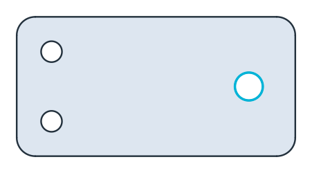
The name of the face becomes the material of the mesh, and the names of its edges become the boundary names, so the names are given before meshing (see Names and colors). The holes come with the layer name holes from the drawing, renamed here to bolts, and the pin hole is the largest of them, Max("radius"), with a name of its own (Figure 2). See Picking what to measure for selections like this.

bracket.name = "steel"
bracket.edges(name="holes").name = "bolts"
bracket.edges(name="bolts").Max("radius").name = "pin"
print(sorted({e.name for e in bracket.edges}))
# px.Plot(bracket)

['bolts', 'outline', 'pin']

Figure 2: The boundaries named for the simulation

See Naming and marking for the other ways to select and name edges.

Meshing

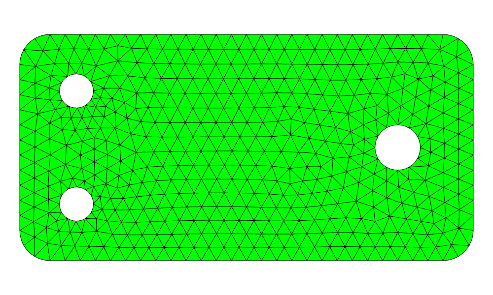
px.OCCGeometry passes the face to netgen with its names, and netgen meshes it with elements of at most 4 mm (see netgen and NGSolve for the installation). Curve(3) places the element edges on the arcs, so that the area of the mesh comes within about 10⁻⁶ of the face’s. The material and the boundary names arrive as they were given. netgen meshes the face here, and gmsh takes the same face just as easily through WriteGeo, which writes a .geo file with the edge names as physical groups (see gmsh and FEniCSx).

mesh = ngs.Mesh(px.OCCGeometry(bracket).GenerateMesh(maxh=0.004))
mesh.Curve(3)
print(mesh.ne, "elements |", mesh.GetMaterials(), "|", sorted(set(mesh.GetBoundaries())))
print("mesh area", ngs.Integrate(1, mesh), "| face area", bracket.mass)
Draw(mesh)

954 elements | ('steel',) | ['bolts', 'outline', 'pin']
mesh area 0.0069047246892775934 | face area 0.006904730091834054

▶ Click to interact

See Meshing a face for mesh sizes on single edges, several regions and refinement towards a corner.

Other formats

The workflow is the same for every format that holds a part’s outline. Only the reader changes:

Format	Reader	See
DXF	px.FromDXF(path, layers=..., unit=..., tol=...)	Files
SVG	px.FromSVG(path)	SVG files
STEP, BREP (planar)	px.FromStep(path), px.FromBrep(path)	STEP and BREP
KiCad, Altium, Eagle and other boards	px.FromKiCad(path)	KiCad, Altium, Eagle and more
Shapely	px.FromShapely(geometry)	Shapely
.CATPart sketches	px.FromCATPart(path)	CATIA V5

Pitfalls

• Units. The readers return meters, and tol and netgen’s maxh are in meters too. Elements of 4 mm in a part drawn in millimeters take maxh=0.004, not 4. A drawing whose header names no unit is read as meters, with a warning, and unit=px.mm sets the unit instead. See Units.

• Layers. Center lines, dimensions and title blocks are lines in the drawing as well. Left in, they cross the part, and px.Face refuses the drawing or makes a different region. layers keeps only the part’s own layers.

• Gaps and small edges. tol closes gaps that are smaller than it. Larger gaps, doubled lines and very short edges need a cleanup first. See Small gaps and Defeaturing and simplification.

• Curved boundaries. Without mesh.Curve(order), the elements have straight edges along the arcs, and the mesh is slightly smaller than the part.

In the browser

The contour checker finds open contours, gaps, doubled lines and small edges in a DXF, SVG or STEP file in the browser, and repairs them, before the file goes into a script. The converters turn DXF, SVG and STEP files into each other.