The skin effect

Why does an alternating current flow near the surface of a wire? The current’s changing magnetic field induces eddy currents in the conductor, which oppose the current in the middle and add to it at the surface. The current density decays inward over the skin depth \(\delta = \sqrt{2/(\omega\mu\sigma)}\), which for copper is 9.3 mm at 50 Hz and 0.21 mm at 100 kHz. In a round wire of radius \(a\), the current density follows a Bessel function, \(J(r) \propto J_0(kr)\) with \(k = (1 - i)/\delta\), and the resistance rises over the direct current’s by

\[\frac{R_{ac}}{R_{dc}} = \operatorname{Re} \frac{ka\,J_0(ka)}{2\,J_1(ka)}.\]

Here, NGSolve solves for the current in a copper wire of 1 mm radius and checks both against the Bessel solution. A flat bar of nearly the same area follows, for which no closed form exists.

import math

import matplotlib.pyplot as plt
import ngsolve as ngs
import numpy as np
import planex as px
from scipy.special import jv

The equations

In the cross-section, the magnetic vector potential \(A\) along the conductor satisfies \(-\nabla \cdot (\mu_0^{-1} \nabla A) + i\omega\sigma A = \sigma E\) in the copper, and the same without the right-hand side and the \(\sigma\) term in the air. \(E = 1\,\text{V/m}\) is the field along the conductor that drives the current, and the current density is \(J = \sigma (E - i\omega A)\). The resistance per meter follows from the power that the current dissipates, \(R = \int |J|^2/\sigma\,dA \,/\, |I|^2\), and the direct current’s is \(1/(\sigma A_{cu})\) for the copper’s area \(A_{cu}\).

section glues the conductor into a circle of air of radius 20 mm, with a fine mesh along the conductor’s edges, and current solves for one frequency:

sigma, mu0 = 5.8e7, 4e-7 * math.pi


def section(conductor):
    conductor.name = "copper"
    conductor.edges.maxh = 2.5e-5
    air = px.Circle((0, 0), 0.02).Face()
    air.name = "air"
    air.edges.name = "outer"
    mesh = ngs.Mesh(px.OCCGeometry(px.Glue([air, conductor])).GenerateMesh(maxh=5e-4))
    mesh.Curve(3)
    return mesh


def current(mesh, f):
    omega = 2 * math.pi * f
    copper = mesh.Materials("copper")
    V = ngs.H1(mesh, order=3, complex=True, dirichlet="outer")
    u, v = V.TnT()
    K = ngs.BilinearForm(ngs.grad(u) * ngs.grad(v) / mu0 * ngs.dx
                         + 1j * omega * sigma * u * v * ngs.dx(definedon=copper)).Assemble()
    F = ngs.LinearForm(sigma * v * ngs.dx(definedon=copper)).Assemble()
    A = ngs.GridFunction(V)
    A.vec.data = K.mat.Inverse(V.FreeDofs(), inverse="umfpack") * F.vec
    J = sigma * (1 - 1j * omega * A)
    I = ngs.Integrate(J, mesh, definedon=copper)
    loss = ngs.Integrate(ngs.Norm(J) ** 2 / sigma, mesh, definedon=copper)
    area = ngs.Integrate(1, mesh, definedon=copper)
    return J, loss / abs(I) ** 2 * sigma * area

A round wire

The wire has a radius of 1 mm. From 50 Hz to 100 kHz, the skin depth falls from more than nine times the radius to a fifth of it, and the resistance ratio follows the Bessel formula:

r0 = 1e-3
wire = section(px.Circle((0, 0), r0).Face())
profiles = {}
for f in (50, 1e3, 1e4, 1e5):
    J, ratio = current(wire, f)
    k = (1 - 1j) * math.sqrt(math.pi * f * mu0 * sigma)
    exact = (k * r0 * jv(0, k * r0) / (2 * jv(1, k * r0))).real
    profiles[f] = (J, k)
    print("f", f, "Hz | skin depth", round(math.sqrt(2) / abs(k) * 1e3, 3), "mm | R_ac/R_dc", ratio, "exact", exact)

f 50 Hz | skin depth 9.346 mm | R_ac/R_dc 1.0000027306955532 exact 1.0000027306955535
f 1000.0 Hz | skin depth 2.09 mm | R_ac/R_dc 1.0010913270688986 exact 1.0010913270665562
f 10000.0 Hz | skin depth 0.661 mm | R_ac/R_dc 1.1005233275603918 exact 1.1005233224735007
f 100000.0 Hz | skin depth 0.209 mm | R_ac/R_dc 2.6616331204101145 exact 2.6616327178051686

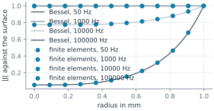
Across the wire, the current density at 50 Hz is nearly uniform. At 100 kHz it falls steeply from the surface, to about an eighth of its value halfway to the center, and the computed densities lie on the Bessel solution (Figure 1):

Figure 1: The current density across a copper wire of 1 mm radius

A flat bar

A flat bar of 3.5 × 0.9 mm has nearly the wire’s area, 3.15 mm² against 3.14 mm², but almost half again its perimeter, 8.8 mm against 6.3 mm. At 100 kHz, its current gathers at the two narrow ends and most of all at the corners (Figure 2), and its resistance rises less:

flat = px.QuickSketch().RectangleC(3.5e-3, 0.9e-3).Face()
bar = section(flat)
J, ratio = current(bar, 1e5)
print("flat bar at 100 kHz: R_ac/R_dc", ratio, "| round wire", current(wire, 1e5)[1])

flat bar at 100 kHz: R_ac/R_dc 2.4299421388433498 | round wire 2.6616331204101145

Figure 2: The current density at 100 kHz