The squircle and the superellipse

What makes a squircle look smoother than a rounded square? A superellipse is the curve

\[\left|\frac{x}{a}\right|^n + \left|\frac{y}{b}\right|^n = 1,\]

which Gabriel Lamé studied. With \(n\) = 2 it is an ellipse, and as \(n\) grows it fills out towards the rectangle around it. Piet Hein chose \(n\) = 2.5 for the Sergels torg roundabout in Stockholm, and the squircle, with \(a = b\) and \(n\) = 4, is used for app icons and in product design. Its area is known in closed form,

\[A = 4ab \, \frac{\Gamma(1 + 1/n)^2}{\Gamma(1 + 2/n)}.\]

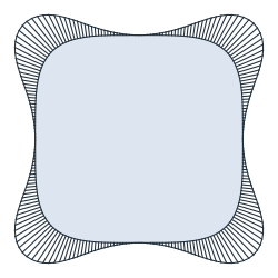
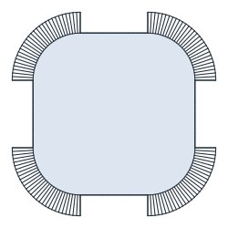
A rounded square of the same size looks almost the same, but its curvature jumps from zero on the side to \(1/r\) on the corner arc. That jump shows in the reflections on a glossy surface. The squircle has no straight part and no jump, and its curvature is zero only at the middle of each side and largest at the diagonals.

The example draws superellipses with px.Curve and checks their areas, reads the squircle’s curvature from its spline and checks it against the exact formula, and compares it with the rounded square of the same area, with arc corners and with curvature-continuous corners.

This page is part of a collection of geometry and design examples using planex2d.

Open this example in the playground, the interactive code editor in the browser, to change the code and run it.

import math

import matplotlib.pyplot as plt
import numpy as np
import planex as px
from scipy.interpolate import BSpline
from scipy.optimize import brentq

Superellipses

A superellipse is drawn from its polar form, in which the point at the angle \(t\) lies at the distance \(r(t) = \left(|\cos t / a|^n + |\sin t / b|^n\right)^{-1/n}\) from the center. One turn of \(t\) gives one closed spline edge, and the area of its face matches the formula to about 1e-10 (Figure 1):

def superellipse(n, a=1, b=1):
    """the face inside |x/a|^n + |y/b|^n = 1"""
    def point(t):
        r = (abs(math.cos(t) / a) ** n + abs(math.sin(t) / b) ** n) ** (-1 / n)
        return (r * math.cos(t), r * math.sin(t))
    return px.Face([px.Curve(point, (0, 2 * math.pi))])


def area(n, a=1, b=1):
    return 4 * a * b * math.gamma(1 + 1 / n) ** 2 / math.gamma(1 + 2 / n)


shapes = {n: superellipse(n) for n in (2, 2.5, 4, 10)}
for n, face in shapes.items():
    print("n", n, "| edges", len(face.edges), "| area", face.mass, "| formula", area(n))
hein = superellipse(2.5, 1.2, 1)
print("Piet Hein's 6 by 5, n 2.5: area", hein.mass, "| formula", area(2.5, 1.2, 1))
# px.Plot(px.Compound(list(shapes.values())))

n 2 | edges 1 | area 3.1415926533929457 | formula 3.1415926535897936
n 2.5 | edges 1 | area 3.380935362207924 | formula 3.380935362537384
n 4 | edges 1 | area 3.708149354682355 | formula 3.708149354602745
n 10 | edges 1 | area 3.942927898014577 | formula 3.9429278978100313
Piet Hein's 6 by 5, n 2.5: area 4.057122434786421 | formula 4.057122435044861

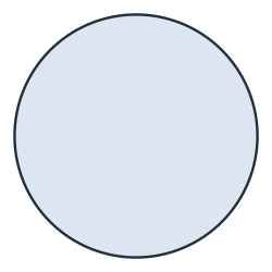
(a) n = 2

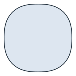
(b) n = 2.5

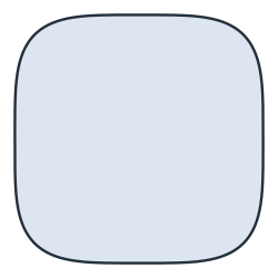
(c) n = 4

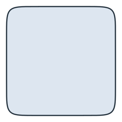
(d) n = 10

Figure 1: Superellipses with a = b = 1, from the circle to almost a square

Their curvature

The curvature of a spline follows from its exact B-spline, as on the page on curvature-continuous blends. The function below goes along a face’s outline, edge by edge, and returns points on it, the unit normals pointing out and the curvature there. The curvature is zero on a line and \(1/r\) on an arc, and on a spline it follows from the first and second derivatives:

def along(face, m=100):
    """points along the outline, the unit normals pointing out and the curvature, m per edge"""
    points, tangents, curvatures = [], [], []
    for e in face.edges:
        edge = e.edge
        if isinstance(edge, px.SplineEdge):
            data = edge.bspline
            p, knots = data["degree"], np.asarray(data["knots"])
            curve = BSpline(knots, np.asarray(data["poles"]), p)
            u = np.linspace(knots[p], knots[-p - 1], m)
            xy, d1, d2 = curve(u), curve.derivative(1)(u), curve.derivative(2)(u)
            speed = np.hypot(d1[:, 0], d1[:, 1])
            t, k = d1 / speed[:, None], (d1[:, 0] * d2[:, 1] - d1[:, 1] * d2[:, 0]) / speed**3
        elif isinstance(edge, px.ArcEdge):
            c, r, turn = np.array([edge.center[0], edge.center[1]]), edge.radius, 1 if edge.ccw else -1
            a0, a1 = (math.atan2(q[1] - c[1], q[0] - c[0]) for q in (edge.start, edge.end))
            a = np.linspace(a0, a0 + turn * ((turn * (a1 - a0)) % (2 * math.pi)), m)
            xy = c + r * np.c_[np.cos(a), np.sin(a)]
            t, k = turn * np.c_[-np.sin(a), np.cos(a)], np.full(m, turn / r)
        else:
            s, f = np.array([edge.start[0], edge.start[1]]), np.array([edge.end[0], edge.end[1]])
            xy = s + np.linspace(0, 1, m)[:, None] * (f - s)
            t, k = np.tile((f - s) / np.hypot(*(f - s)), (m, 1)), np.zeros(m)
        points.append(xy)
        tangents.append(t)
        curvatures.append(k)
    t = np.vstack(tangents)
    return np.vstack(points), np.c_[t[:, 1], -t[:, 0]], np.concatenate(curvatures)

On the superellipse itself, the curvature at a point \((x, y)\) is

\[\kappa = \frac{(n - 1) \, |x y|^{n - 2}}{\left(|x|^{2n - 2} + |y|^{2n - 2}\right)^{3/2}},\]

which is zero on the axes for \(n > 2\) and \((n - 1) \, 2^{1/n - 1/2}\) at the diagonals. The squircle’s spline follows it:

squircle = shapes[4]
xy, normals, kappa = along(squircle, 2000)
x, y = np.abs(xy[:, 0]), np.abs(xy[:, 1])
exact = 3 * (x * y) ** 2 / (x**6 + y**6) ** 1.5
print("largest curvature", kappa.max(), "| at the diagonals", 3 * 2 ** (1 / 4 - 1 / 2))
print("smallest", kappa.min(), "| largest difference from the formula", np.abs(kappa - exact).max())

largest curvature 2.5227144830552835 | at the diagonals 2.5226892457611436
smallest -0.0001609302322962541 | largest difference from the formula 0.0001609302322962541

Against a rounded square

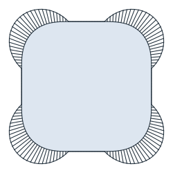
A square of side 2 with corner arcs of radius \(r\) has the area \(4 - (4 - \pi) r^2\), so the rounded square with the squircle’s area has \(r\) = 0.583. The same square with curvature-continuous (G2) corners, made with Filleted and px.Curvature, has its own area, and SciPy’s brentq finds the radius that gives it the squircle’s area too. The arc corners stay within 0.017 of the squircle and the G2 corners within 0.010:

square = px.QuickSketch().RectangleC((0, 0), 2, 2).Face()
r_arc = math.sqrt((4 - area(4)) / (4 - math.pi))
r_g2 = brentq(lambda r: square.Filleted(square.vertices, r, px.Curvature).mass - area(4), 0.3, 0.99, xtol=1e-14)
arcs = square.Filleted(square.vertices, r_arc)
g2 = square.Filleted(square.vertices, r_g2, px.Curvature)
for name, face, r in (("arcs", arcs, r_arc), ("curvature-continuous", g2, r_g2)):
    print(name, "| r", r, "| area", face.mass, "| Hausdorff distance from the squircle", face.Hausdorff(squircle))

arcs | r 0.5830873454143245 | area 3.7081493546027446 | Hausdorff distance from the squircle 0.016516239148364815
curvature-continuous | r 0.7235772064207657 | area 3.7081493546027433 | Hausdorff distance from the squircle 0.009840534375391173

The differences show in the curvature. A curvature comb, as CAD systems draw it, puts a line along the normal at each point of the outline, as long as the curvature there. The arc corners’ comb steps from zero to \(1/r\) where the side ends, the curvature-continuous corners rise from zero, and the squircle’s comb has no step and no straight part (Figure 2):

def comb(face, m, scale=0.15):
    """the curvature comb of the outline: the teeth along the normals and the line through their tips"""
    xy, normals, kappa = along(face, m)
    tips = xy + scale * kappa[:, None] * normals
    teeth = [px.Line(tuple(p), tuple(q)) for p, q in zip(xy, tips) if np.hypot(*(q - p)) > 1e-9]
    keep = np.r_[True, np.hypot(*np.diff(tips, axis=0).T) > 1e-9]
    return px.Compound(teeth + [px.FromPolyline(tips[keep], closed=True)])


combs = {"Squircle": (squircle, 240), "Arc corners": (arcs, 30), "G2 corners": (g2, 30)}
# px.Plot(px.Compound([squircle, comb(squircle, 240)]))

(a) Squircle

(b) Arc corners

(c) G2 corners

Figure 2: Curvature combs of the squircle and of the rounded square of the same area

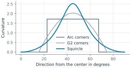
Along a quarter of the outline, the curvature of the arc corners jumps twice, at the directions where the corners start and end. The G2 corners, of radius 0.724, peak at a curvature of 2.03, and the squircle peaks at 2.52 on its diagonal (Figure 3):

quarter = {}
for name, (face, m) in combs.items():
    xy, normals, kappa = along(face, 8 * m)
    direction = np.degrees(np.arctan2(xy[:, 1], xy[:, 0])) % 360
    order = np.argsort(direction, kind="stable")
    keep = order[direction[order] <= 90]
    quarter[name] = (direction[keep], kappa[keep])
    print(name, "| largest curvature", kappa.max())
# plt.plot(*quarter["Squircle"]); plt.show()

Squircle | largest curvature 2.522712054722941
Arc corners | largest curvature 1.715008922530174
G2 corners | largest curvature 2.0316632679492566

Figure 3: The curvature along a quarter of the outline

See Curves from equations for px.Curve and Curvature-continuous blends for Fillet with px.Curvature.