Stress at a shoulder fillet

How sharp may the shoulder of a stepped bar be? Where a bar steps down from the width \(D\) to the width \(d\), the stress in the inside corner rises above the nominal stress in the narrow part, by the stress concentration factor \(K_t\). A sharp corner has no finite \(K_t\) at all, and a fillet of radius \(r\) brings it down, the more the larger it is. Designers read \(K_t\) from Peterson’s charts, which give it over \(r/d\) for each ratio \(D/d\).

The example draws the bar as a parametric sketch whose fillet radius and widths are dimensions, and solves it in plane stress with NGSolve for several radii. \(K_t\) must agree with Peterson’s charts, and it must grow without bound as the fillet gets sharper.

import math

import ngsolve as ngs
import planex as px

The bar

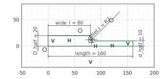
The bar is symmetric about its axis, so the sketch is its upper half, with the axis along \(x\). The narrow part is \(d = 20\) wide and the wide part \(D = 40\), each 80 long, and the fillet in the shoulder’s corner has the radius \(r = 2\). Every line is level or plumb and is drawn so, and auto_constraint={"horizontal": True, "vertical": True} keeps it so. The half widths, the lengths and the fillet’s radius fillet.r are the dimensions. The edges that the solve needs carry names: axis on the axis, load at the narrow end and end at the wide end (Figure 1):

bar = px.Sketch(auto_constraint={"horizontal": True, "vertical": True})
bar.Move((0, 0)).Line(160, id="axis", name="axis")
bar.Turn(90).Line(10, id="load", name="load")
bar.Turn(90).Line(80, id="narrow")
bar.Turn(-90).Line(10, id="shoulder")
bar.Turn(90).Line(80, id="wide")
bar.Close(id="end", name="end")
bar.Constrain("axis.start", "origin", px.Coincident)
bar.Constrain("axis", px.Distance, 160, id="length")
bar.Constrain("wide", px.Distance, 80, id="wide_l")
bar.Constrain("narrow", "H", px.Distance, 20 / 2, id="d_half")
bar.Constrain("wide", "H", px.Distance, 40 / 2, id="D_half")
bar.Fillet(["narrow.end"], 2, id="fillet")
print("status", bar.status, "| degrees of freedom", bar.dof)

status full | degrees of freedom 0

Figure 1: The stepped bar as a parametric sketch

Tension

The narrow end carries a tension of 1 per unit of area, so the nominal stress in the narrow part is 1, and the peak stress is \(K_t\). The wide end is held along \(x\) and the axis across it, as the bar’s symmetry requires. solve meshes the face, with a mesh size of \(r/16\) along the fillet, and solves plane-stress linear elasticity with NGSolve, with fifth-order elements on a curved mesh. On the free edges, the only stress is the one along the edge, the trace of the stress tensor, and solve returns its largest value there. Young’s modulus and Poisson’s ratio do not change the stresses:

def solve(face, r, order=5):
    """the stress field and the peak stress along the free edges of the half bar"""
    for edge in face.edges:
        if edge.name is None:
            edge.name = "free"
        if abs(edge.mass - math.pi * r / 2) < 1e-9:
            edge.maxh = r / 16
    mesh = ngs.Mesh(px.OCCGeometry(face).GenerateMesh(maxh=5))
    mesh.Curve(order)
    fes = ngs.VectorH1(mesh, order=order, dirichletx="end", dirichlety="axis")
    u, v = fes.TnT()
    E, nu = 210e3, 0.3
    mu, lam = E / 2 / (1 + nu), E * nu / (1 - nu**2)

    def stress(w):
        e = ngs.Sym(ngs.Grad(w))
        return 2 * mu * e + lam * ngs.Trace(e) * ngs.Id(2)

    a = ngs.BilinearForm(ngs.InnerProduct(stress(u), ngs.Sym(ngs.Grad(v))) * ngs.dx).Assemble()
    f = ngs.LinearForm(v[0] * ngs.ds("load")).Assemble()
    gf = ngs.GridFunction(fes)
    gf.vec.data = a.mat.Inverse(fes.FreeDofs(), inverse="sparsecholesky") * f.vec
    sigma = ngs.Trace(stress(gf))
    rule = ngs.IntegrationRule(ngs.SEGM, 2 * order + 2)
    along = ngs.BoundaryFromVolumeCF(sigma)(mesh.MapToAllElements(rule, mesh.Boundaries("free"))).flatten()
    return sigma, mesh, along.max()


sigma, mesh, Kt = solve(bar.Face(), 2)
print("D/d 2 | r/d 0.1 | Kt", Kt)

D/d 2 | r/d 0.1 | Kt 2.5056575774328

The sum of the principal stresses is 1 in the narrow part and \(\tfrac{1}{2}\) in the wide part, far from the shoulder, and on the fillet’s edge it peaks at \(K_t\). Around the shoulder:

Against the body force method

Noda, Kanemoto, Nisitani and Fujisaki computed \(K_t\) for stepped flat bars in tension with the body force method, a boundary integral method, to three or four digits. They tabulate it over the step’s share of the wide width, \(2h/D\), where \(h = (D - d)/2\) is the height of the step, and over \(h/r\). With \(r = h/2\), the bars below go from a small step, \(2h/D = 0.1\), to a step half as high as the bar, \(2h/D = 0.5\). Update sets the wide part’s half width and the fillet’s radius together, and the solver keeps every other dimension. \(K_t\) is compared with their values:

noda = {0.1: 2.504, 0.2: 2.356, 0.3: 2.197, 0.4: 2.028, 0.5: 1.849}  # Kt by 2h/D, for h/r = 2
for step, value in noda.items():
    D = 20 / (1 - step)
    r = (D - 20) / 4
    bar.Update({"D_half": D / 2, "fillet.r": r})
    print("D/d", round(D / 20, 3), "| r/d", round(r / 20, 4), "| Kt", round(solve(bar.Face(), r)[2], 4),
          "| body force method", value)

D/d 1.111 | r/d 0.0278 | Kt 2.4996 | body force method 2.504
D/d 1.25 | r/d 0.0625 | Kt 2.3517 | body force method 2.356
D/d 1.429 | r/d 0.1071 | Kt 2.1939 | body force method 2.197
D/d 1.667 | r/d 0.1667 | Kt 2.0262 | body force method 2.028
D/d 2.0 | r/d 0.25 | Kt 1.8482 | body force method 1.849

The two methods agree within 0.2 %.

Against Peterson’s chart

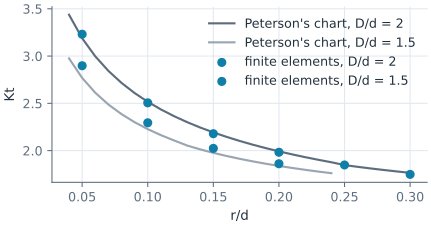
Peterson’s chart for this bar goes back to photoelastic measurements. Pilkey fitted it as \(K_t = C_1 + C_2\,(2h/D) + C_3\,(2h/D)^2 + C_4\,(2h/D)^3\), with each coefficient of the form \(a + b\sqrt{h/r} + c\,h/r\), one set of \(a\), \(b\) and \(c\) for \(h/r\) up to 2 and another from 2 to 20. \(K_t\) for \(D/d = 2\) and 1.5 and \(r/d\) from 0.05 to 0.3, as far as the fillet fits into the step, is compared with the fit:

FIT = {False: [(1.006, 1.008, -0.044), (-0.115, -0.584, 0.315), (0.245, -1.006, -0.257), (-0.135, 0.582, -0.017)],
       True: [(1.020, 1.009, -0.048), (-0.065, -0.165, -0.007), (-3.459, 1.266, -0.016), (3.505, -2.109, 0.069)]}


def peterson(D, d, r):
    """Kt of a stepped flat bar in tension from the fit of Peterson's chart; FIT[True] for h/r above 2"""
    h = (D - d) / 2
    return sum((a + b * math.sqrt(h / r) + c * h / r) * (2 * h / D) ** k for k, (a, b, c) in enumerate(FIT[h / r > 2]))


results = {}
for D in (40, 30):
    results[D] = []
    for rd in (0.05, 0.1, 0.15, 0.2, 0.25, 0.3):
        r = rd * 20
        if r < (D - 20) / 2:
            bar.Update({"D_half": D / 2, "fillet.r": r})
            results[D].append((rd, solve(bar.Face(), r)[2]))
            print("D/d", D / 20, "| r/d", rd, "| Kt", round(results[D][-1][1], 4), "| chart", round(peterson(D, 20, r), 4))

D/d 2.0 | r/d 0.05 | Kt 3.2312 | chart 3.1892
D/d 2.0 | r/d 0.1 | Kt 2.5057 | chart 2.5164
D/d 2.0 | r/d 0.15 | Kt 2.1791 | chart 2.1927
D/d 2.0 | r/d 0.2 | Kt 1.9828 | chart 1.9922
D/d 2.0 | r/d 0.25 | Kt 1.8482 | chart 1.8469
D/d 2.0 | r/d 0.3 | Kt 1.7488 | chart 1.765
D/d 1.5 | r/d 0.05 | Kt 2.898 | chart 2.7691
D/d 1.5 | r/d 0.1 | Kt 2.2947 | chart 2.2272
D/d 1.5 | r/d 0.15 | Kt 2.0238 | chart 1.9764
D/d 1.5 | r/d 0.2 | Kt 1.8612 | chart 1.8381

For \(D/d = 2\), the finite elements and the chart agree within 1.5 %, and at the sharpest fillet the finite elements lie higher. For \(D/d = 1.5\), they lie up to 5 % above the chart, which Noda and his coauthors found to underestimate \(K_t\) by about 10 % in places. As \(r/d\) goes to zero, both grow without bound (Figure 2).

Figure 2: The stress concentration factor of a stepped flat bar in tension

See Changing dimensions for Update and the airplane windows for the stress around holes and sharp corners.