Views of solids

px.Drawing(part, plane) draws an OpenCASCADE solid as it is seen along a plane:

Plane	The view
px.Front, px.Top, px.Left, px.Right, px.Rear, px.Bottom	The six standard views, named “Front view”, “Top view” and so on
px.Plane(...)	An auxiliary view, seen from the side its normal points to, named “Auxiliary view”
px.Isometric	A shaded pictorial, named “Isometric view”

Visible edges and the outlines of curved faces, their fold lines, are drawn wide, and hidden edges narrow and dashed. Smooth edges, where two faces meet tangentially, are drawn narrow and stop short of the outline. hidden=False leaves the hidden edges out, and view_name= replaces a view’s name, or removes it with "". dw.Add(sk) puts the dimensions of a constraint sketch on a view, and px.Sheet places the views in first-angle projection, as for drawings of sketches. The edges come from OpenCASCADE’s exact hidden-line algorithm, and the fold lines it traces only approximately are refined onto the exact surfaces.

import math
import netgen.occ as occ
import planex as px

A bearing plate in three views

The example is the bearing plate of A dimensioned drawing, padded to a thickness of 10, with a hub of diameter 48 and 15 high around its bore. px.Pad makes the plate from its sketch, and a second pad on the plate’s top face makes the hub, whose outer face gets the name hub (see Pad and Pocket). The volume is the plate’s area times its thickness, plus the ring of the hub:

part = px.Pad(plate, 10)
top = part.faces.Max(occ.Z)
part = part + px.Pad(px.QuickSketch(top).Circle((0, 0), 24, name="hub").Circle((0, 0), 20), 15)
print("volume", part.mass, "exact", plate.Face().mass * 10 + math.pi * (24**2 - 20**2) * 15)

volume 88633.36324000738 exact 88633.36324000762

The front view shows the bore and the bolt holes as hidden edges. The top view carries the dimensions of the plate’s sketch, and the left view and the isometric complete the sheet, an A4 sheet laid on its side. Two lengths that no sketch holds, the thickness of the plate and the height of the hub, are added to the front view with Measure, in the view’s own coordinates, \(x\) to the right and \(z\) up:

front = px.Drawing(part, px.Front, unit=px.mm)
front.Measure((60, 0), (60, 10)).Measure((24, 10), (24, 25))
top_view = px.Drawing(part, px.Top, unit=px.mm).Add(plate)
left = px.Drawing(part, px.Left, unit=px.mm)
iso = px.Drawing(part, px.Isometric, unit=px.mm)
px.Sheet(front, top_view, left, iso, landscape=True)

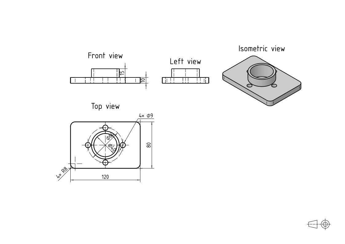
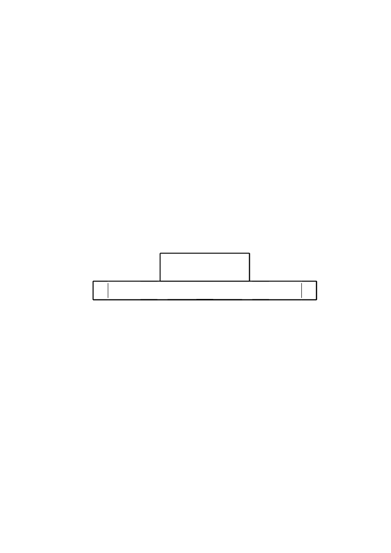
Without its hidden edges and its name, the front view shows only what is seen:

px.Drawing(part, px.Front, unit=px.mm, hidden=False, view_name="")

Curved faces and rounded edges

A curved face has no edge where it turns away from the viewer, but a view shows its outline there, the fold line, drawn wide like an edge. A rounded edge leaves two smooth edges, where the round meets its two faces tangentially, and these are drawn narrow and stop short of the outline. The example rounds the outer edge of the hub’s top with a radius of 2. That edge is the edge of the face hub above \(z = 24.9\), and MakeFillet of netgen.occ rounds it:

rim = part.faces["hub"].edges[occ.Z > 24.9]
rounded = part.MakeFillet(rim, 2)

The round removes a ring whose cross-section is a corner square of side \(r\) less a quarter circle, \(r^2 (1 - \pi/4)\), with its centroid \(\tfrac{10 - 3\pi}{12 - 3\pi}\,r\) inside the corner, which lies 24 from the axis. By Pappus’s rule, the ring’s volume is its cross-section times the path of its centroid:

\[V = 2\pi \left(24 - \frac{10 - 3\pi}{12 - 3\pi}\,r\right) r^2 \left(1 - \frac{\pi}{4}\right)\]

r = 2
ring = 2 * math.pi * (24 - (10 - 3 * math.pi) / (12 - 3 * math.pi) * r) * r**2 * (1 - math.pi / 4)
print("volume", rounded.mass, "exact", part.mass - ring)

volume 88506.32794621393 exact 88506.32794621393

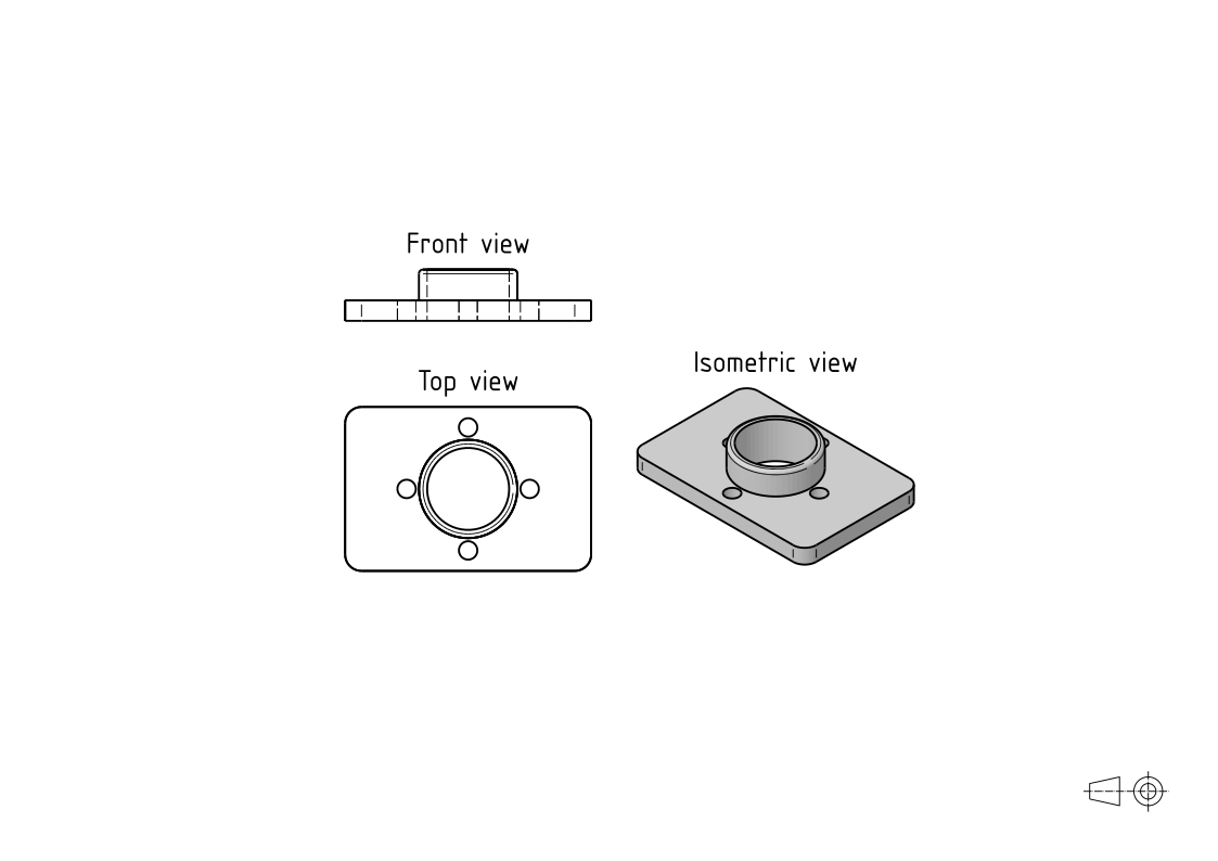
In the front view, the hub’s top corners are round, and a narrow line marks where the round meets the hub’s wall. In the top view, the narrow circle inside the hub’s outline is where the round meets the hub’s top face:

front = px.Drawing(rounded, px.Front, unit=px.mm)
top_view = px.Drawing(rounded, px.Top, unit=px.mm)
sheet = px.Sheet(front, top_view, landscape=True)
sheet.Add(px.Drawing(rounded, px.Isometric, unit=px.mm), at=(150, -80))
sheet

A view square to a slope

The example is the block of the exercise Inclined block, built as on that page. It is 80 long and 45 high at its left end and 20 at its right, and its slope falls at 30° from the top. A counterbore of 11, 6.5 deep, and a hole of 6.6 go into the slope square to it, sketched on the slope. The front view shows the slope as a line and the top view shows it foreshortened, so only a view square to the slope shows the face and its hole as they are. Such an auxiliary view is a drawing seen along a plane of its own.

The plane view_a lies in the slope, its origin at the slope’s lower end in front, its normal the slope’s, out of the block, and its \(h\) axis along \(y\). The sketches of the counterbore and the hole lie in this plane, so Add puts their dimensions on the view at their true lengths. hidden=False leaves the hidden edges out, and the counterbore’s depth, which no sketch holds, follows its diameter as “↧6,5”:

t = math.radians(30)
normal = (math.sin(t), 0, math.cos(t))
(x0, z0), (x1, z1) = profile.Location("slope.start")[:2], profile.Location("slope.end")[:2]
view_a = px.Plane(origin=(x0, 0, z0), normal=normal, axis=(0, 1, 0))
a_view = px.Drawing(block, view_a, unit=px.mm, view_name="A", hidden=False).Add(counterbore).Add(hole)
a_view.Place("counterbore_d", suffix="↧6,5")

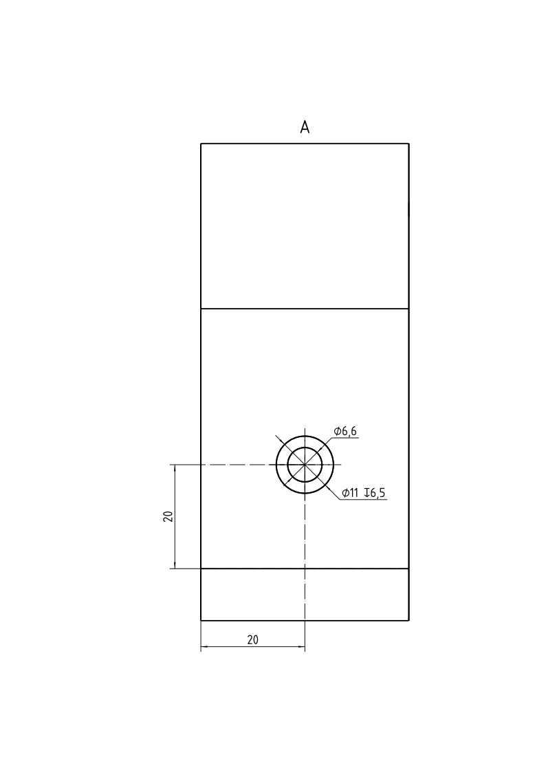
On the front view, Callout marks where view A is seen from, with an arrow at the slope that points into it. The front view takes its place on the sheet, and Add puts view A at 140 to the right of the front view’s origin, on the side it is seen from:

front_view = px.Drawing(block, px.Front, unit=px.mm).Add(profile).Place("slope_angle", 22)
tip = (x0 + 0.3 * (x1 - x0) + 3 * normal[0], z0 + 0.3 * (z1 - z0) + 3 * normal[2])
front_view.Callout(tip, (-normal[0], -normal[2]), "A")
sheet = px.Sheet(front_view, landscape=True)
sheet.Add(a_view, at=(140, -5))
sheet

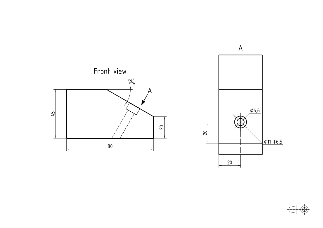
The slope’s face in view A is as high as the slope is long, \(25 / \sin 30^\circ\), the difference of the two ends’ heights over the sine of its angle:

print("slope", profile.Measure("slope")["length"], "exact", 25 / math.sin(t))

slope 50.00000000000001 exact 50.00000000000001

See Sections for a view cut at a plane, and Views and sheets for views drawn from sketches.