Drawing with epicycles

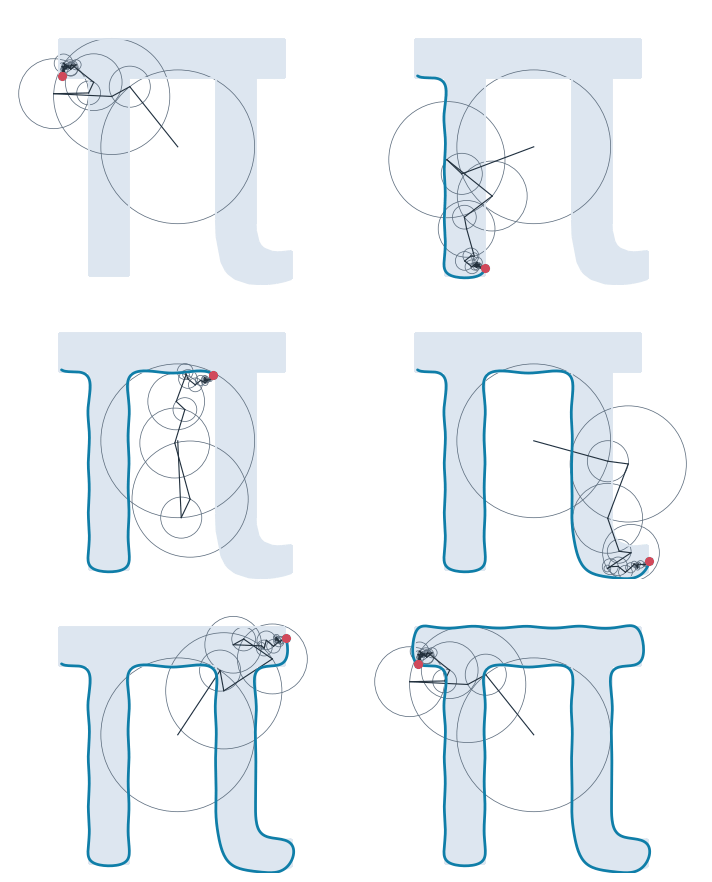
How can a chain of circles, each turning at its own constant speed, draw the letter π? Any closed curve, written as a complex number \(z(t)\) that runs once around it as \(t\) goes from 0 to 1, is a Fourier series,

\[z(t) = \sum_n c_n e^{2\pi i n t}.\]

Each term is a circle of radius \(|c_n|\) turned \(n\) times per lap, carried on the circle before it, like the deferent and the epicycle of the old planetary models. Kept to the terms with \(|n| \le K\), the chain of \(2K + 1\) circles draws a curve that comes closer to the outline as \(K\) grows. The area that the curve encloses follows from the coefficients alone, by Green’s theorem,

\[A = \pi \sum_n n \, |c_n|^2.\]

It is positive for a curve that runs counterclockwise.

The example takes the outline of the letter from matplotlib’s font, computes its coefficients with NumPy’s FFT, draws the curves of the circle chains with px.Curve and compares planex2d’s exact area of each curve with the formula.

This page is part of a collection of geometry and design examples using planex2d.

Open this example in the playground, the interactive code editor in the browser, to change the code and run it.

import numpy as np
from matplotlib.font_manager import FontProperties
from matplotlib.textpath import TextPath
import planex as px

The outline

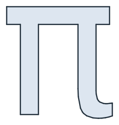
The letter is taken from DejaVu Sans, the font that comes with matplotlib, at a size of 100. Its outline is one closed polygon, reversed so that it runs counterclockwise (Figure 1):

path = TextPath((0, 0), "π", size=100, prop=FontProperties(family="DejaVu Sans"))
outline = path.to_polygons()[0][:-1][::-1]
letter = px.FromPolyline(outline, closed=True).Face()
print("area", letter.mass, "| edges", len(letter.edges))
# px.Plot(letter)

area 1370.2235050201416 | edges 33

Figure 1: The outline to draw

The coefficients

The outline is sampled at 2048 points spaced evenly along its length. The FFT of the samples, divided by their number, gives the coefficients \(c_n\) for \(n\) from \(-1024\) to \(1023\). The term \(c_0\) is the center of the outline, the point the chain starts from:

closed = np.vstack([outline, outline[:1]])
length = np.concatenate([[0], np.cumsum(np.hypot(*np.diff(closed, axis=0).T))])
spaced = np.linspace(0, length[-1], 2048, endpoint=False)
z = np.interp(spaced, length, closed[:, 0]) + 1j * np.interp(spaced, length, closed[:, 1])
c = np.fft.fft(z) / len(z)
n = np.fft.fftfreq(len(z), 1 / len(z))
print("center", c[0], "| largest circle", abs(c[1:]).max())

center (31.135363145144552+29.844201120865367j) | largest circle 17.75423905122192

The chain of circles

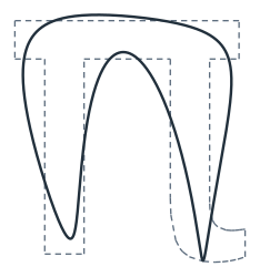
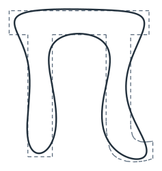
The function below adds the terms with \(|n| \le K\) at \(t\) and draws the curve they trace from \(t = 0\) to 1 with px.Curve. It also returns the area from the coefficients, which is compared with planex2d’s area of the face inside the curve (Figure 2):

def chain(K):
    """the curve that the 2K + 1 circles with |n| <= K draw, and its area from the coefficients"""
    keep = abs(n) <= K

    def point(t):
        w = np.sum(c[keep] * np.exp(2j * np.pi * n[keep] * t))
        return (w.real, w.imag)

    return px.Curve(point, (0, 1)), np.pi * np.sum(n[keep] * abs(c[keep]) ** 2)


curves = {}
for K in (3, 6, 12, 25):
    curves[K], area = chain(K)
    print("K", K, "|", 2 * K + 1, "circles | area", px.Face([curves[K]]).mass, "| from the coefficients", area)
# px.Plot(curves[25])

K 3 | 7 circles | area 1307.3194849284448 | from the coefficients 1307.319484774471
K 6 | 13 circles | area 1323.2729101847071 | from the coefficients 1323.2729100103677
K 12 | 25 circles | area 1363.9681688962405 | from the coefficients 1363.9681689717308
K 25 | 51 circles | area 1371.3408395289778 | from the coefficients 1371.340839490385

(a) K = 3: 7 circles

(b) K = 6: 13 circles

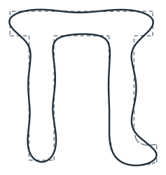
(c) K = 12: 25 circles

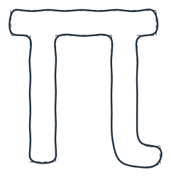
(d) K = 25: 51 circles

Figure 2: The curves of four chains, the letter dashed

Closer with more circles

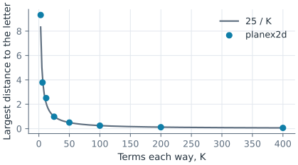
How close a curve comes to the letter is the largest distance between the two, their Hausdorff distance. With many circles the curve has fine detail, so here it is drawn through 4000 of its points as a polyline. The distance falls about as \(1/K\), because a curve with corners has coefficients that fall as \(1/n^2\), and the corners are the last to come close (Figure 3):

t = np.linspace(0, 1, 4000, endpoint=False)
Ks = [3, 6, 12, 25, 50, 100, 200, 400]
distances = []
for K in Ks:
    keep = abs(n) <= K
    w = np.exp(2j * np.pi * np.outer(t, n[keep])) @ c[keep]
    polyline = px.FromPolyline(np.column_stack([w.real, w.imag]), closed=True)
    distances.append(letter.wires[0].Hausdorff(polyline))
print("K", Ks)
print("distance", [round(d, 3) for d in distances])
print("K times distance", [round(K * d, 1) for K, d in zip(Ks, distances)])
# px.Plot(polyline)

K [3, 6, 12, 25, 50, 100, 200, 400]
distance [9.323, 3.785, 2.506, 0.981, 0.501, 0.246, 0.119, 0.061]
K times distance [28.0, 22.7, 30.1, 24.5, 25.0, 24.6, 23.7, 24.6]

Figure 3: The Hausdorff distance between the curve and the letter

See Curves from equations for px.Curve.