Chladni figures

What do the sand patterns on a bowed plate show? Ernst Chladni strewed sand on metal plates and bowed their edges. At each natural frequency, the plate vibrates in one of its modes, and the sand gathers on the nodal lines, where the plate stands still. The frequencies of a square plate free at all its edges are tabulated as the coefficients \(\lambda^2 = \omega a^2 \sqrt{\rho h / D}\), with \(a\) the side, \(h\) the thickness, \(\rho\) the density and \(D = E h^3 / (12 (1 - \nu^2))\) the bending stiffness. For \(\nu = 0.3\), the first are 13.463, 19.596, 24.270, 34.788 (twice) and 61.090 (twice), as Apaipong and Sompornjaroensuk list them, in agreement with Leissa’s classic tables.

Here, NGSolve finds the modes of a thin square plate, the frequencies are checked against the coefficients, and the nodal lines are drawn.

import math

import ngsolve as ngs
import numpy as np
import planex as px
import scipy.sparse as sp
from scipy.sparse.linalg import eigsh

The plate

The plate is a square of side 1, 0.002 thick, with \(E = 1\), \(\rho = 1\) and \(\nu = 0.3\), so the coefficients come out directly. It bends as a Reissner-Mindlin plate: the deflection \(w\) and the rotations \(\theta\) are unknowns of their own, coupled by the shear \(\nabla w - \theta\). For a plate this thin, the model approaches the classic thin plate. Nothing holds the edges, so they are free:

a, h, E, nu, rho = 1.0, 0.002, 1.0, 0.3, 1.0
D, G = E * h**3 / (12 * (1 - nu**2)), E / (2 * (1 + nu))
plate = px.QuickSketch().RectangleC(a, a).Face()
mesh = ngs.Mesh(px.OCCGeometry(plate).GenerateMesh(maxh=a / 12))

X = ngs.H1(mesh, order=6) * ngs.VectorH1(mesh, order=5)
(w, th), (v, et) = X.TnT()
bend = ngs.Sym(ngs.Grad(th)), ngs.Sym(ngs.Grad(et))
stiff = D * ((1 - nu) * ngs.InnerProduct(*bend) + nu * ngs.div(th) * ngs.div(et)) \
    + 5 / 6 * G * h * (ngs.grad(w) - th) * (ngs.grad(v) - et)
mass = rho * h * w * v + rho * h**3 / 12 * th * et
stiffness, inertia = ngs.BilinearForm(stiff * ngs.dx).Assemble(), ngs.BilinearForm(mass * ngs.dx).Assemble()
K = sp.csr_matrix(stiffness.mat.CSR(), shape=(X.ndof, X.ndof))  # the forms stay alive: CSR() shares their memory
M = sp.csr_matrix(inertia.mat.CSR(), shape=(X.ndof, X.ndof))

The frequencies

SciPy’s eigsh finds the lowest modes. The first three have no frequency: the plate moves up and down or tilts as a whole, without bending. The next ones are the Chladni modes, and their coefficients agree with the table to about four digits:

values, vectors = eigsh(K, k=12, M=M, sigma=-1e-6, which="LM")
order = np.argsort(values)
values, vectors = values[order], vectors[:, order]
table = [13.463, 19.596, 24.270, 34.788, 34.788, 61.090, 61.090, 63.655, 69.241]
for value, listed in zip(values[3:], table):
    print("λ²", round(math.sqrt(value) * a**2 * math.sqrt(rho * h / D), 3), "| table", listed)

λ² 13.465 | table 13.463
λ² 19.596 | table 19.596
λ² 24.27 | table 24.27
λ² 34.792 | table 34.788
λ² 34.792 | table 34.788
λ² 61.09 | table 61.09
λ² 61.09 | table 61.09
λ² 63.664 | table 63.655
λ² 69.247 | table 69.241

The nodal lines

On a grid over the plate, the deflection \(w\) of a mode changes its sign across the nodal lines, which are drawn in dark, the deflection in color (Figure 1). Where two modes share a frequency, any combination of them vibrates at it as well, and the solver returns one of them:

mode = ngs.GridFunction(X)
grid = np.linspace(-a / 2, a / 2, 121) * (1 - 1e-9)
gh, gv = np.meshgrid(grid, grid)


def deflection(k):
    mode.vec.FV().NumPy()[:] = vectors[:, k]
    shape = np.asarray(mode.components[0](mesh(gh.ravel(), gv.ravel()))).reshape(gh.shape)
    return shape / np.abs(shape).max()

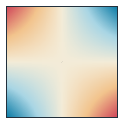
(a) λ² = 13.46

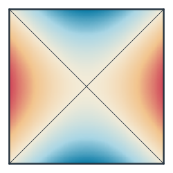
(b) λ² = 19.60

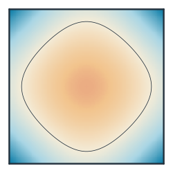
(c) λ² = 24.27

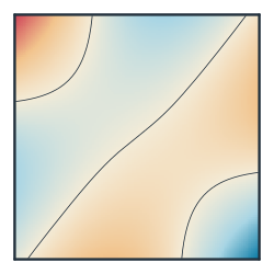
(d) λ² = 34.79

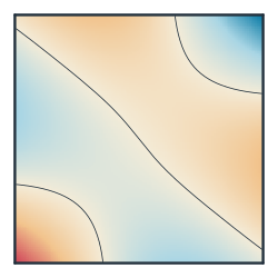
(e) λ² = 34.79

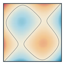
(f) λ² = 61.09

Figure 1: Six modes of a free square plate and their nodal lines