The Joukowski airfoil

How much lift does a wing section give? In potential flow, the Kutta-Joukowski theorem gives the lift per unit span as \(L' = \rho U \Gamma\), the density times the speed times the circulation \(\Gamma\) around the section. The Kutta condition fixes the circulation: the flow leaves the sharp trailing edge smoothly instead of turning around it. For a Joukowski airfoil, the image of a circle under the conformal map \(z = \zeta + b^2/\zeta\), the circulation is exact:

\[\Gamma = 4\pi U a \sin(\alpha + \beta),\]

with \(a\) the circle’s radius, \(\alpha\) the angle of attack and \(\beta\) the angle at which the circle passes through \(\zeta = b\), the point that becomes the trailing edge. The lift coefficient is \(C_L = 2\Gamma/(U c)\) for the chord \(c\).

Here, px.Curve draws the airfoil exactly from its map, NGSolve solves the potential flow around it, and the circulation is checked against the exact one.

import math

import ngsolve as ngs
import numpy as np
import planex as px

The airfoil

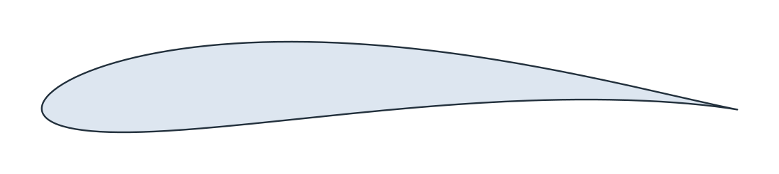
The circle has its center at \((-0.1, 0.1)\) and passes through \(\zeta = b = 1\), so its radius is \(a = \sqrt{1.1^2 + 0.1^2}\) and \(\beta = \arctan(0.1/1.1)\). The real part of its center makes the airfoil thick and the imaginary part cambers it. With \(\zeta = (-0.1 + a\cos t) + i\,(0.1 + a\sin t)\), the map gives the airfoil as two expression strings in \(t\), starting at the trailing edge, \(t = -\beta\) (Figure 1):

b = 1.0
mx = 0.1
my = 0.1
a = math.hypot(b + mx, my)
beta = math.atan2(my, b + mx)
u = f"(-{mx} + {a}*cos(t))"
v = f"({my} + {a}*sin(t))"
x = f"{u} + {b * b}*{u}/({u}^2 + {v}^2)"
y = f"{v} - {b * b}*{v}/({u}^2 + {v}^2)"
start = -math.degrees(beta)
foil = px.Curve((x, y), (start, start + 360))
(x0, _), (x1, _) = foil.bounding_box
chord = x1 - x0
print("chord", chord, "| trailing edge at", x1)

chord 4.0336016535116075 | trailing edge at 2.0

Figure 1: A cambered Joukowski airfoil

The flow

The stream function \(\psi\) of a potential flow satisfies \(\nabla^2 \psi = 0\), and the airfoil, which the flow does not cross, has a constant \(\psi\) on it. Far away, on a circle of radius 50, the flow is uniform at the angle of attack. The solution is the uniform flow around the airfoil, \(\psi_s\) with \(\psi = 0\) on the airfoil, plus a multiple of the pure circulation, \(\psi_c\) with \(\psi = 1\) on the airfoil and 0 far away:

body = px.Face([foil])
body.edges.name = "foil"
body.edges.maxh = 0.01
air = px.Circle((0, 0), 50).Face()
air.edges.name = "far"
mesh = ngs.Mesh(px.OCCGeometry((air - body).Face()).GenerateMesh(maxh=5, grading=0.2))
mesh.Curve(3)
V = ngs.H1(mesh, order=3, dirichlet="far|foil")
p, q = V.TnT()
K = ngs.BilinearForm(ngs.grad(p) * ngs.grad(q) * ngs.dx).Assemble()
inverse = K.mat.Inverse(V.FreeDofs(), inverse="umfpack")


def potential(far, on_foil):
    psi = ngs.GridFunction(V)
    psi.Set(mesh.BoundaryCF({"far": far, "foil": on_foil}), ngs.BND)
    psi.vec.data += inverse * (-K.mat * psi.vec)
    return psi

The Kutta condition

A flow that turned around the sharp trailing edge would do so at an infinite speed. The Kutta condition picks the multiple \(k\) of \(\psi_c\) for which the flow just behind the cusp runs along the trailing edge’s direction, the angle \(-2\beta\), instead of across it. The circulation is then the flux of \(\nabla\psi\) through the airfoil’s outline:

edge = np.array([x1, 0.0])
along = np.array([math.cos(-2 * beta), math.sin(-2 * beta)])
across = np.array([-along[1], along[0]])
behind = edge + 3e-4 * along
normal = ngs.specialcf.normal(2)


def velocity(psi):
    gx, gy = ngs.grad(psi)(mesh(*behind))
    return np.array([gy, -gx])


for alpha in (0, 4, 8):
    rad = math.radians(alpha)
    stream, circulation = potential(ngs.cos(rad) * ngs.y - ngs.sin(rad) * ngs.x, 0), potential(0, 1)
    k = -(velocity(stream) @ across) / (velocity(circulation) @ across)
    gamma = abs(ngs.Integrate(ngs.BoundaryFromVolumeCF(ngs.grad(stream) + k * ngs.grad(circulation)) * normal, mesh,
                              ngs.BND, definedon=mesh.Boundaries("foil")))
    exact = 4 * math.pi * a * math.sin(rad + beta)
    print("α", alpha, "° | Γ", round(gamma, 5), "exact", round(exact, 5), "| C_L", round(2 * gamma / chord, 4),
          "exact", round(2 * exact / chord, 4))

α 0 ° | Γ 1.25856 exact 1.25664 | C_L 0.624 exact 0.6231
α 4 ° | Γ 2.22098 exact 2.21782 | C_L 1.1012 exact 1.0997
α 8 ° | Γ 3.17257 exact 3.1682 | C_L 1.5731 exact 1.5709

The circulation and the lift come within 0.2 % of the exact values, and the lift grows with the angle of attack as \(\sin(\alpha + \beta)\). At zero angle of attack, the camber alone gives lift. The streamlines at 8° leave the trailing edge smoothly: