The slider-crank and the Scotch yoke

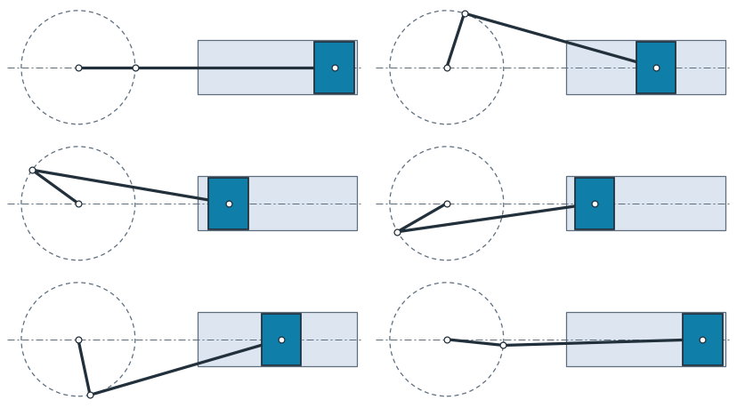
Does a piston move like a pendulum? Its crank turns evenly, but the connecting rod tilts as it turns, and the piston position for a crank of radius \(r\) and a rod of length \(l\) at the crank angle \(\theta\) is

\[x = r \cos\theta + \sqrt{l^2 - r^2 \sin^2\theta}.\]

That is not a pure cosine. The piston moves faster near the top of its stroke than near the bottom. Its acceleration is \(r \omega^2 (1 + r/l)\) at the top and \(r \omega^2 (1 - r/l)\) at the bottom, and its motion has a second harmonic of about \(r^2 / 4l\) at twice the crank speed. That harmonic is the second-order shaking of four-cylinder inline engines, which some of them cancel with balance shafts turning at twice the crank speed. The Scotch yoke drives its slide with a slotted yoke instead of a rod, and the slide moves as a pure cosine, \(x = r \cos\theta\).

The example draws both mechanisms as constraint sketches with the crank angle as a dimension, turns them through a full revolution, and checks the piston against the formula, its accelerations, and the harmonics of its motion.

This page is part of a collection of mechanism examples using planex2d.

Open this example in the playground, the interactive code editor in the browser, to change the code and run it.

import math

import matplotlib.pyplot as plt
import numpy as np
import planex as px
from scipy.integrate import quad

The two mechanisms

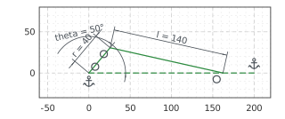
The crank is 40 long and turns about the origin, which gives a stroke of 80, in millimeters. In the slider-crank, a rod of 140 runs from the crank pin to the piston pin, which stays on the cylinder’s axis. These are about the proportions of a car engine. The crank angle is the dimension theta between the axis and the crank:

r, l = 40, 140


def slider_crank(theta=50):
    """the crank at theta degrees to the cylinder's axis, and the rod to the piston pin on the axis"""
    t = math.radians(theta)
    sk = px.Sketch()
    sk.Move((0, 0), px.Fix).Line(200, 0, id="axis", construction=True)
    sk.Constrain("axis.end", px.Fix)
    sk.Move("axis.start", px.Coincident).Line(r * math.cos(t), r * math.sin(t), id="crank")
    sk.Move("crank.end", px.Coincident).Line(130, -20, id="rod")
    sk.Constrain("rod.end", "axis", px.Coincident)
    sk.Constrain("crank", px.Distance, r, id="r")
    sk.Constrain("rod", px.Distance, l, id="l")
    sk.Constrain("axis", "crank", px.Angle, theta, id="theta")
    return sk


crank = slider_crank()
print("slider-crank:", crank.status, "| degrees of freedom", crank.dof, "| piston pin", crank.Location("rod.end")[:2])
# crank.Plot(show_constraints=True)

slider-crank: full | degrees of freedom 0 | piston pin (162.3170732998103, 3.572395989835586e-18)

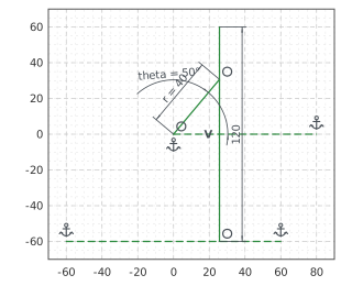
In the Scotch yoke, the crank pin slides in a vertical slot, 120 long, whose foot runs on a rail below the axis. Figure 1 shows both sketches with their constraints:

def scotch_yoke(theta=50):
    """the crank at theta degrees to the axis, its pin in a vertical slot whose foot runs on a rail"""
    t = math.radians(theta)
    sk = px.Sketch()
    sk.Move((0, 0), px.Fix).Line(80, 0, id="axis", construction=True)
    sk.Constrain("axis.end", px.Fix)
    sk.Move((-60, -60), px.Fix).Line(120, 0, id="rail", construction=True)
    sk.Constrain("rail.end", px.Fix)
    sk.Move("axis.start", px.Coincident).Line(r * math.cos(t), r * math.sin(t), id="crank")
    sk.Move((r * math.cos(t), -60)).Line(0, 120, id="slot")
    sk.Constrain("slot.start", "rail", px.Coincident)
    sk.Constrain("crank.end", "slot", px.Coincident)
    sk.Constrain("slot", px.Vertical)
    sk.Constrain("slot", px.Distance, 120)
    sk.Constrain("crank", px.Distance, r, id="r")
    sk.Constrain("axis", "crank", px.Angle, theta, id="theta")
    return sk


yoke = scotch_yoke()
print("Scotch yoke:", yoke.status, "| degrees of freedom", yoke.dof, "| slot at", yoke.Location("slot.start")[0])
# yoke.Plot(show_constraints=True)

Scotch yoke: full | degrees of freedom 0 | slot at 25.711504387461574

(a) The slider-crank

(b) The Scotch yoke

Figure 1: Both mechanisms with the crank at 50°

A full turn

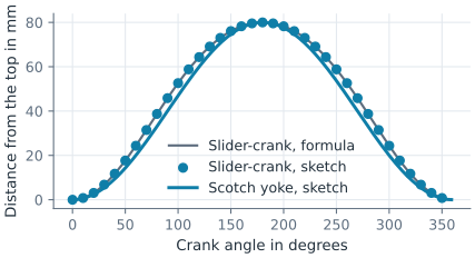
Update turns the crank one degree at a time, and each sketch solves for the rest. The piston follows the formula, and the yoke’s slot follows a pure cosine:

angles = np.arange(360)
piston, slot = [], []
for theta in angles:
    crank.Update({"theta": float(theta)})
    yoke.Update({"theta": float(theta)})
    piston.append(crank.Location("rod.end")[0])
    slot.append(yoke.Location("slot.start")[0])
piston, slot = np.array(piston), np.array(slot)
t = np.radians(angles)
formula = r * np.cos(t) + np.sqrt(l**2 - r**2 * np.sin(t) ** 2)
print("slider-crank, largest difference from the formula", np.abs(piston - formula).max())
print("Scotch yoke, largest difference from r cos θ", np.abs(slot - r * np.cos(t)).max())

slider-crank, largest difference from the formula 8.526512829121202e-14
Scotch yoke, largest difference from r cos θ 3.6415315207705135e-14

In the first quarter turn, the piston covers \(r + l - \sqrt{l^2 - r^2}\), more than half its stroke, while the yoke covers exactly half (Figure 2):

print("after a quarter turn: piston", piston[0] - piston[90], "of", piston[0] - piston[180],
      "| formula", r + l - math.sqrt(l**2 - r**2), "| yoke", slot[0] - slot[90])
# plt.plot(angles, piston[0] - piston, angles, slot[0] - slot); plt.show()

after a quarter turn: piston 45.8359213500126 of 80.0 | formula 45.835921350012626 | yoke 40.0

Figure 2: The piston and the yoke over a full turn

Animate plays the slider-crank through the same turn, a frame every 6°, and writes the piston’s position into each frame:

crank.Animate({"theta": np.arange(0, 360, 6)}, fps=20, label=lambda s: "piston at %.1f" % s.Location("rod.end")[0])

Accelerations and harmonics

The piston’s acceleration over \(\omega^2\) is the second derivative of its position by the crank angle. Taken from the sketch at a tenth of a degree on either side of the top and the bottom, it matches \(r (1 \pm r/l)\):

def acceleration(theta, h=0.1):
    """the second derivative of the piston position by the crank angle, from the sketch"""
    x = []
    for d in (-h, 0, h):
        crank.Update({"theta": (theta + d) % 360})
        x.append(crank.Location("rod.end")[0])
    return (x[0] - 2 * x[1] + x[2]) / math.radians(h) ** 2


print("top", acceleration(0), "| formula", -r * (1 + r / l))
print("bottom", acceleration(180), "| formula", r * (1 - r / l))

top -51.42855038867777 | formula -51.42857142857142
bottom 28.571429327141317 | formula 28.571428571428573

The Fourier series of the piston position over a turn shows the rod’s effect. The first harmonic is exactly the crank radius, the odd ones above it vanish, and the second is close to \(r^2 / 4l\). Its exact amplitude is the integral of the formula against \(\cos 2\theta\). The yoke has the first harmonic only:

harmonics, yoke_harmonics = (np.abs(np.fft.rfft(x)) / len(x) * 2 for x in (piston, slot))
def second(a):
    return (r * math.cos(a) + math.sqrt(l**2 - r**2 * math.sin(a) ** 2)) * math.cos(2 * a)


exact = quad(second, 0, 2 * math.pi)[0] / math.pi
print("slider-crank harmonics 1 to 6", np.round(harmonics[1:7], 9))
print("second: exact", exact, "| r²/4l", r**2 / (4 * l))
print("Scotch yoke harmonics 1 to 6", np.round(yoke_harmonics[1:7], 9))

slider-crank harmonics 1 to 6 [4.0000000e+01 2.9177954e+00 0.0000000e+00 1.5526341e-02 0.0000000e+00
 1.6524400e-04]
second: exact 2.9177953982412053 | r²/4l 2.857142857142857
Scotch yoke harmonics 1 to 6 [40.  0.  0.  0.  0.  0.]

See Changing dimensions for Update, Animating a sketch for Animate and The four-bar linkage for another mechanism turned through a full revolution.