Turing patterns

Why can a spotted animal have a ringed tail? Alan Turing showed that two substances that react with each other and diffuse at different rates can turn a uniform mixture into a pattern. The uniform state is unstable to waves of one band of wavelengths, and the waves that grow fastest set the spacing of the spots or stripes that form. James Murray took this as a model of the markings on an animal’s coat and found that the shape of the skin decides the pattern. A tail so thin that no wave around it can grow carries only rings. A spotted animal can therefore have a ringed tail, as the cheetah and the genet have, but a striped animal cannot have a spotted one.

The example uses Schnakenberg’s model, one of the standard two-substance reactions. Its linear analysis gives the growth rate of every wavelength. NGSolve and SciPy then let a pattern grow from a little noise on a square, where the growth rates of the waves are checked against the analysis, and on the skin of a tapering tail, unrolled flat, where the spots give way to rings at the circumference the analysis predicts.

This page is part of a collection of field and simulation examples using planex2d.

import math

import matplotlib.pyplot as plt
import ngsolve as ngs
import numpy as np
import planex as px
import scipy.sparse as sp
from scipy.fft import dctn
from scipy.optimize import minimize_scalar
from scipy.sparse.linalg import splu

The growth rates

The two concentrations \(u\) and \(v\) react and diffuse as

\[\frac{\partial u}{\partial t} = a - u + u^2 v + \nabla^2 u, \qquad \frac{\partial v}{\partial t} = b - u^2 v + d \, \nabla^2 v,\]

in the model’s own units of length and time. With \(a\) = 0.1, \(b\) = 0.9 and \(v\) diffusing \(d\) = 20 times as fast as \(u\), the uniform state \(u_0 = a + b\), \(v_0 = b / (a + b)^2\) is stable without diffusion. A small wave of wavenumber \(k\) on it grows at the rate of the larger eigenvalue of \(J - k^2 \operatorname{diag}(1, d)\), where \(J\) is the Jacobian of the reactions. It grows where the determinant of that matrix is negative, between the two roots \(k^2 = \left(p \pm \sqrt{p^2 - 4 d \det J}\right) / 2d\) with \(p = d J_{11} + J_{22}\):

a, b, d = 0.1, 0.9, 20
u0, v0 = a + b, b / (a + b) ** 2
J = np.array([[2 * u0 * v0 - 1, u0**2], [-2 * u0 * v0, -(u0**2)]])


def growth(k):
    """the growth rate of a wave with the wavenumber k on the uniform state"""
    return np.linalg.eigvals(J - k**2 * np.diag([1, d])).real.max()


kmax = minimize_scalar(lambda k: -growth(k), bounds=(0.1, 1), method="bounded", options={"xatol": 1e-10}).x
p = d * J[0, 0] + J[1, 1]
k1, k2 = (math.sqrt((p + s * math.sqrt(p**2 - 4 * d * np.linalg.det(J))) / (2 * d)) for s in (-1, 1))
wavelength = 2 * math.pi / kmax
print("fastest-growing wavenumber", kmax, "| rate", growth(kmax), "| wavelength", wavelength)
print("growing from k =", k1, "to", k2, "| shortest growing wavelength", 2 * math.pi / k2)

fastest-growing wavenumber 0.48666425609197306 | rate 0.2631578947368425 | wavelength 12.910718690612338
growing from k = 0.271956127951169 to 0.8222164340791343 | shortest growing wavelength 7.641765655312675

Spots on a square

The square is ten wavelengths across, meshed by netgen with triangle sides of at most a twelfth of a wavelength. Each time step takes the diffusion implicitly, with the mass matrix lumped onto the vertices, and the reactions explicitly, so that the two matrices are factored once. A face with identified edges gets NGSolve’s Periodic space, which the tail below needs. The run starts from the uniform state with a noise of a millionth and returns \(u\) at the times asked for:

def simulate(face, times, dt=0.1, seed=1):
    """the mesh and u at the given times, grown from the uniform state with a little noise"""
    mesh = ngs.Mesh(px.OCCGeometry(face).GenerateMesh(maxh=wavelength / 12))
    V = ngs.H1(mesh, order=1)
    if face.identifications:
        V = ngs.Periodic(V)
    trial, test = V.TnT()
    free = np.flatnonzero(V.FreeDofs())

    def matrix(form):
        m = ngs.BilinearForm(form).Assemble().mat
        return sp.csr_matrix(m.CSR(), shape=(V.ndof, V.ndof))[free][:, free]

    M = np.asarray(matrix(trial * test * ngs.dx).sum(axis=1)).ravel()
    K = matrix(ngs.grad(trial) * ngs.grad(test) * ngs.dx)
    solve_u, solve_v = (splu((sp.diags(M) + dt * D * K).tocsc()).solve for D in (1, d))
    rng = np.random.default_rng(seed)
    u, v = (c * (1 + 1e-6 * rng.standard_normal(len(free))) for c in (u0, v0))
    found, t = [], 0.0
    for T in times:
        while t < T - dt / 2:
            uuv = u * u * v
            u, v = solve_u(M * (u + dt * (a - u + uuv))), solve_v(M * (v + dt * (b - uuv)))
            t += dt
        found.append(ngs.GridFunction(V))
        found[-1].vec.FV().NumPy()[free] = u
    return mesh, found


side = round(10 * wavelength)
square = px.QuickSketch().Rectangle(side, side).Face()
mesh, (early, later, emerging, settled) = simulate(square, (5, 15, 50, 800))
print(mesh.ne, "triangles")

33332 triangles

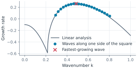
On a square with insulated sides, every pattern is a sum of cosine waves, and while the pattern is small each wave grows on its own. The cosine coefficients of \(u\), taken on a grid of 256 by 256 points, give each wave’s growth rate between the times 5 and 15. The waves along one side lie on the curve of the analysis (Figure 1):

def cosines(g, n=256):
    """the squared cosine coefficients of u on the square and their wavenumbers"""
    x = (np.arange(n) + 0.5) * side / n
    gx, gy = np.meshgrid(x, x)
    values = np.asarray(g(mesh(gx.ravel(), gy.ravel()))).reshape(n, n)
    m = np.arange(n) * math.pi / side
    return np.hypot(*np.meshgrid(m, m)), dctn(values, norm="ortho") ** 2


k, before = cosines(early)
_, after = cosines(later)
measured = np.log(after / before) / (2 * (15 - 5))
waves = (k[0] > k1) & (k[0] < k2)
predicted = np.array([growth(q) for q in k[0][waves]])
fast = predicted > 0.1
print(waves.sum(), "growing waves along one side; where faster than 0.1, largest difference",
      np.abs(measured[0][waves] - predicted)[fast].max())
# plt.plot(k[0][waves], measured[0][waves], "o"); plt.show()

22 growing waves along one side; where faster than 0.1, largest difference 0.00902355300165232

Figure 1: The growth rate of every wavelength

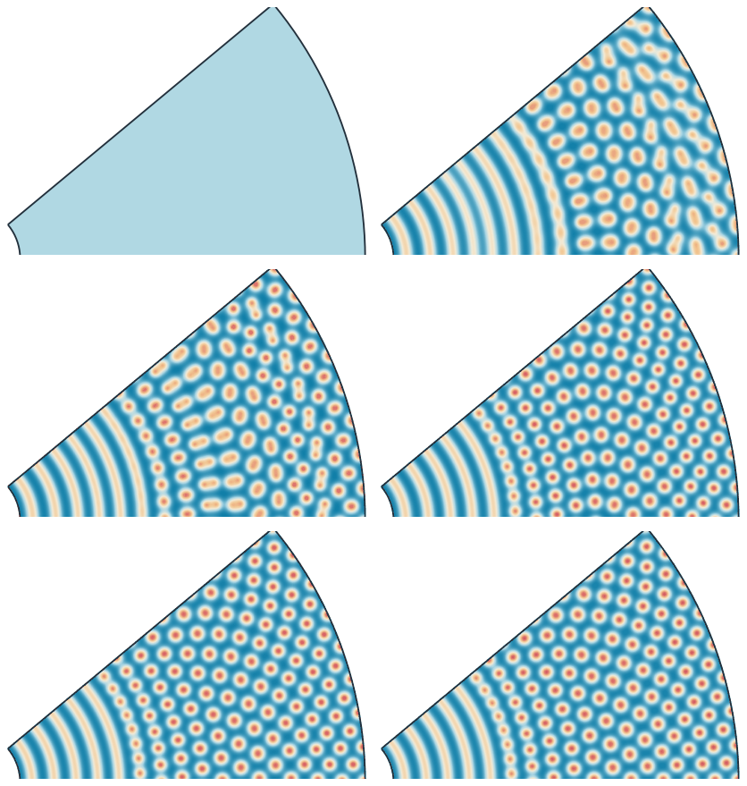
Once the waves are large, the reactions couple them, and they settle into a hexagonal pattern of spots (Figure 2). The settled spots lie closer together than the wavelength that grew fastest, though still inside the band of growing wavenumbers:

k, power = cosines(settled)
power[0, 0] = 0
print("strongest wavenumber at the end", k.ravel()[power.argmax()], "| fastest-growing", kmax)
# px.PlotField(settled, mesh, square)

strongest wavenumber at the end 0.5445592814760252 | fastest-growing 0.48666425609197306

(a) At the time 50

(b) At the time 800

Figure 2: Spots growing out of noise on the square, and the settled pattern

A tapering tail

A tail is close to a cone, and the skin of a cone unrolls flat into a sector of a ring without stretching, so that diffusion on it is diffusion on the flat sector. The two straight sides of the sector are the same line on the tail, and identifying them closes the skin. The tail is 15 wavelengths long, 1.5 wavelengths around at the root and a fifth of one at the tip:

around_root, around_tip, length = 1.5 * wavelength, 0.2 * wavelength, 15 * wavelength
turn = (around_root - around_tip) / length
r_tip = around_tip / turn


def sector(turns=1):
    """the skin of the tail unrolled, or several turns of it side by side"""
    sk = px.QuickSketch((r_tip, 0)).Line(length, name="side_a")
    sk.Arc(center=(0, 0), sweep=turns * math.degrees(turn), name="root").Turn(90).Line(length, name="side_b")
    return sk.Arc(center=(0, 0), sweep=-turns * math.degrees(turn), name="tip").Face()


tail = sector()
tail.Identify("side_a", "side_b")
print("sector of", math.degrees(turn), "degrees | area", tail.mass,
      "| cone's side", (around_root + around_tip) / 2 * length)
tail_mesh, (skin,) = simulate(tail, (800,))

sector of 4.965634224467134 degrees | area 2125.2548781286046 | cone's side 2125.2548781286164

At each distance from the tip, the circle around the tail shows whether it carries a ring, with the same value all the way around, or spots. The rings end close to where the circumference reaches the shortest wavelength that can grow (Figure 3):

def spread(r):
    """how much u varies around the tail at the radius r of the sector"""
    angle = np.linspace(0, turn, 60)
    values = np.asarray(skin(tail_mesh(r * np.cos(angle), r * np.sin(angle)))).ravel()
    return values.max() - values.min()


radii = np.arange(r_tip + 0.5, r_tip + length / 2, 0.25)
first = next(r for r in radii if spread(r) > 0.1)
print("rings up to the circumference", (first - 0.25) * turn, "| spots from", first * turn,
      "| shortest growing wavelength", 2 * math.pi / k2)
# px.PlotField(skin, tail_mesh, tail)

rings up to the circumference 7.890477071455801 | spots from 7.9121437381224675 | shortest growing wavelength 7.641765655312675

Figure 3: The tail's skin unrolled, its sector drawn eight times around

See Identifications for identified edges and the rotational sector, and Chladni figures for patterns set by the shape of a plate.