The Venturi meter

Why does the pressure drop where a pipe narrows? Where the flow speeds up, part of its pressure has become kinetic energy, and Bernoulli’s equation, \(p + \tfrac{1}{2}\rho u^2 = \text{const}\) along a streamline, says how much. This is the Venturi effect, and the Venturi meter turns it into a flow measurement. From the pressure difference \(\Delta p\) between the pipe and the throat, continuity and Bernoulli’s equation give the flow rate

\[Q_{ideal} = A_2 \sqrt{\frac{2\,\Delta p}{\rho\,\left(1 - (A_2/A_1)^2\right)}}.\]

Bernoulli’s equation neglects viscosity, so the real flow is somewhat less, by the discharge coefficient \(C = Q / Q_{ideal}\). Here, netgen meshes a planar Venturi channel and NGSolve solves the Navier-Stokes equations in it at rising Reynolds numbers. Bernoulli’s equation is checked along the centerline, and the meter’s discharge coefficient comes from its wall taps.

import math

import matplotlib.pyplot as plt
import ngsolve as ngs
import numpy as np
import planex as px
from ngsolve.solvers import Newton

The channel

The channel follows the classical Venturi tube: a convergent of 21°, a throat as long as it is wide, and a slowly widening divergent of 7°, which turns part of the speed back into pressure. It is planar, a width of \(D = 2\) narrowing to \(d = 1\), so the area ratio is \(A_2/A_1 = d/D = 0.5\), where a round tube would have the square of the diameter ratio. Straight pieces of 4 before and 6 after keep the inlet and the outlet away from the contraction. The upper wall is a polyline, the lower one its mirror image, and the eight corners between the pieces are rounded with a radius of 1, as the transitions of a real tube are (Figure 1):

conv = 0.5 / math.tan(math.radians(21 / 2))
div = 0.5 / math.tan(math.radians(7 / 2))
x = np.cumsum([0, 4, conv, 1, div, 6])
upper = [(x[0], 1), (x[1], 1), (x[2], 0.5), (x[3], 0.5), (x[4], 1), (x[5], 1)]
channel = px.Face([px.FromPolyline(upper + [(h, -v) for h, v in reversed(upper)], closed=True)])
channel = channel.Filleted([(h, s * v) for h, v in upper[1:5] for s in (1, -1)], 1)
channel.edges.name = "wall"
channel.edges(near=(x[0], 0)).name = "inlet"
channel.edges(near=(x[5], 0)).name = "outlet"

Figure 1: The planar Venturi channel

The flow

The inlet carries a parabolic profile with a mean velocity of 1, the walls hold the fluid at rest, and the outlet is left free, so the pressure there is zero on average. With the density 1, the Reynolds number of the throat is \(Re = u_2 d / \nu = 2 / \nu\). Newton’s method solves the steady Navier-Stokes equations, each Reynolds number starting from the solution of the one before:

mesh = ngs.Mesh(px.OCCGeometry(channel).GenerateMesh(maxh=0.08))
X = ngs.VectorH1(mesh, order=2, dirichlet="wall|inlet") * ngs.H1(mesh, order=1)
(u, p), (v, q) = X.TnT()
flow = ngs.GridFunction(X)
flow.components[0].Set(ngs.CF((1.5 * (1 - ngs.y**2), 0)), definedon=mesh.Boundaries("inlet"))


def solve(Re):
    nu = 2 / Re
    form = nu * ngs.InnerProduct(ngs.grad(u), ngs.grad(v)) + ngs.InnerProduct(ngs.grad(u) * u, v) \
        - ngs.div(v) * p - ngs.div(u) * q
    Newton(ngs.BilinearForm(form * ngs.dx), flow, freedofs=X.FreeDofs(), maxerr=1e-10, inverse="umfpack",
           printing=False)


print(mesh.ne, "elements")

13236 elements

Bernoulli along the centerline

The pressure taps sit 1 before the convergent and in the middle of the throat. Along the centerline, the total pressure \(p + \tfrac{1}{2}u^2\) would stay the same without viscosity. Its loss from the inlet tap to the throat, measured against the throat’s dynamic pressure, shrinks as the Reynolds number grows. At the walls, the pressure difference gives the meter’s flow rate \(Q_{ideal}\), and the true flow rate is 2, the inlet’s width times its mean velocity:

velocity, pressure = flow.components
inlet_tap, throat_tap = x[1] - 1, (x[2] + x[3]) / 2


def total(s):
    return pressure(mesh(s, 0.0)) + velocity(mesh(s, 0.0))[0] ** 2 / 2


for Re in (20, 100, 200, 400, 800):
    solve(Re)
    loss = (total(inlet_tap) - total(throat_tap)) / (velocity(mesh(throat_tap, 0.0))[0] ** 2 / 2)
    dp = pressure(mesh(inlet_tap, 1 - 1e-6)) - pressure(mesh(throat_tap, 0.5 - 1e-6))
    q_ideal = 1 * math.sqrt(2 * dp / (1 - 0.5**2))
    print("Re", Re, "| Bernoulli loss", round(100 * loss, 1), "% | wall Δp", round(dp, 3), "| C", round(2 / q_ideal, 3))

Re 20 | Bernoulli loss 68.9 % | wall Δp 6.376 | C 0.485
Re 100 | Bernoulli loss 9.3 % | wall Δp 2.95 | C 0.713
Re 200 | Bernoulli loss 4.7 % | wall Δp 2.392 | C 0.792
Re 400 | Bernoulli loss 2.5 % | wall Δp 2.044 | C 0.857
Re 800 | Bernoulli loss 1.3 % | wall Δp 1.816 | C 0.909

The loss about halves with each doubling of the Reynolds number, so the centerline approaches Bernoulli’s equation as viscosity matters less and less in the core of the flow. The wall taps still read more than Bernoulli’s equation gives for the mean velocities, \(\tfrac{1}{2}(2^2 - 1^2) = 1.5\). Near the walls, the fluid is slowed, so the core runs faster than the mean, and the pressure falls further than the mean velocity says. The meter therefore reads too much flow, and its discharge coefficient rises toward 1 as the layers near the walls grow thinner. Real meters run at Reynolds numbers far higher than this laminar flow and are calibrated there.

The pressure along the channel

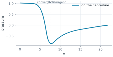
At \(Re = 800\), the pressure on the centerline falls through the convergent, is lowest in the throat, and rises again in the divergent (Figure 2). In this laminar flow, the divergent recovers only part of the drop, since the friction at the walls takes much of it:

recovered = (pressure(mesh(x[4] + 0.2, 1 - 1e-6)) - pressure(mesh(throat_tap, 0.5 - 1e-6))) / dp
print("the divergent recovers", round(100 * recovered), "% of the drop")

the divergent recovers 36 % of the drop

Figure 2: The pressure along the channel at Re 800

The speed is highest in the throat, and the layers of slower fluid near the walls grow along the divergent (Figure 3):

Figure 3: The speed at Re 800