Design tables in a spreadsheet
A design table lists the variants of a part, one row per variant and one column per dimension, as CAD systems keep them in a spreadsheet. A constraint sketch writes such a table and reads it back:
Call |
What it does |
|---|---|
|
Appends the current solution as a row, with its name, every dimension by id, and further values such as an area |
|
Returns the rows as the sketch’s driving dimensions, |
A missing or empty file gets a header row first, and every later row must have the same columns. A CSV file is written with Python’s csv module, with commas between the values and a decimal point. An Excel file, .xlsx, works the same way and needs the optional package openpyxl.
[1]:
import math
from pathlib import Path

import planex as px
Writing the variants
The example is the plate from Constraints and dimensions, \(w\) = 50 by \(h\) = 30 with one corner rounded to a radius \(r\) of 10 and a hole of diameter \(d\) = 10, placed 20 from the left side and 15 from the bottom. Its area is \(w h - (1 - \pi/4)\,r^2 - \pi d^2/4\).
[3]:
plate = px.Sketch(id="plate")
plate.Move(plate.origin, px.Coincident)
plate.Line(37, 2.5, px.Horizontal, id="bottom")
plate.Arc(9, 95, px.Tangent, id="fillet")
plate.Line(-1, 17, px.Vertical, px.Tangent, id="right")
plate.Line(-46, 3, px.Perpendicular, id="top")
plate.Close(px.Perpendicular, id="left")
plate.Constrain("fillet", px.Radius, 10, id="r")
plate.Constrain("bottom.start", "right", px.Distance, 50, id="width")
plate.Constrain("bottom", "top", px.Distance, 30, id="height")
plate.Circle((20, 15), 5, id="hole")
plate.Constrain("hole", px.Diameter, 10, id="d")
plate.Constrain("hole.center", "bottom", px.Distance, 15, id="y_hole")
plate.Constrain("hole.center", "left", px.Distance, 20, id="x_hole")
print(plate.status, plate.dof, "degrees of freedom, dimensions", sorted(plate.dimensions))
full 0 degrees of freedom, dimensions ['d', 'height', 'r', 'width', 'x_hole', 'y_hole']
Three sizes go into the file plates.csv, each with its area as a further column. AddToSpreadsheet appends to a file that exists, so the example starts with an empty one:
[4]:
sizes = {"P50": {"width": 50, "height": 30, "r": 10, "d": 10, "x_hole": 20, "y_hole": 15},
         "P70": {"width": 70, "height": 40, "r": 12, "d": 14, "x_hole": 25, "y_hole": 20},
         "P90": {"width": 90, "height": 50, "r": 15, "d": 18, "x_hole": 30, "y_hole": 25}}
Path("plates.csv").unlink(missing_ok=True)
for name, size in sizes.items():
    plate.Update(size)
    plate.AddToSpreadsheet("plates.csv", name=name, values={"area": plate.Face().mass})
print(Path("plates.csv").read_text())
name,r,width,height,d,y_hole,x_hole,area
P50,10.0,50.0,30.0,10.0,15.0,20.0,1400.0
P70,12.0,70.0,40.0,14.0,20.0,25.0,2615.159295503333
P90,15.0,90.0,50.0,18.0,25.0,30.0,4197.245581823651
Reading them back
ReadSpreadsheet returns every row by its name, with the driving dimensions only. The area is no dimension of the sketch, so it stays out. Update with a row turns the sketch into that variant, and each variant’s area matches the formula (Figure 1):
[5]:
def area(row):
    """the plate's area from its dimensions"""
    return row["width"] * row["height"] - (1 - math.pi / 4) * row["r"] ** 2 - math.pi * row["d"] ** 2 / 4


rows = plate.ReadSpreadsheet("plates.csv")
print(rows["P70"])
variants = {}
for name, row in rows.items():
    variants[name] = plate.Copy().Update(row)
    print(name, "area", variants[name].Face().mass, "exact", area(row))
{'r': 12.0, 'width': 70.0, 'height': 40.0, 'd': 14.0, 'y_hole': 20.0, 'x_hole': 25.0}
P50 area 1400.0 exact 1400.0
P70 area 2615.159295503333 exact 2615.159295503333
P90 area 4197.245581823651 exact 4197.245581823652
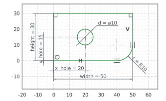
(a) P50
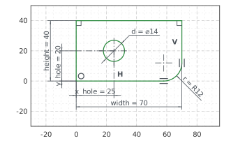
(b) P70
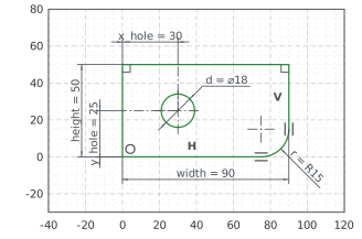
(c) P90
sk.Animate(rows) plays the same rows as an animation. See Animating a sketch for details.