The Helmholtz coil

Why are the two coils of a Helmholtz pair exactly one radius apart? Two equal coils on one axis, carrying the same current the same way, add their fields. In the middle between them, the odd derivatives of the field along the axis vanish by symmetry, and the second derivative vanishes when the spacing equals the radius. The field is then uniform to the fourth order,

\[\frac{B(z)}{B_0} \approx 1 - \frac{144}{125} \left(\frac{z}{R}\right)^4, \qquad B_0 = \left(\frac{4}{5}\right)^{3/2} \frac{\mu_0 n I}{R},\]

for coils of radius \(R\) with \(n\) turns carrying the current \(I\). Such pairs cancel the Earth’s field around an experiment or set up a known field to calibrate magnetic sensors.

The example models two windings of 100 turns each, with a square section of 1 cm on a radius of 15 cm, in the plane through their axis. NGSolve solves for their field, which is checked against the exact field of the windings on the axis, and the field along the axis for three spacings shows why the radius is the right one.

This page is part of a collection of field and simulation examples using planex2d.

import math

import matplotlib.pyplot as plt
import ngsolve as ngs
import numpy as np
import planex as px
from scipy.integrate import dblquad

The coil pair

A coil’s field is the same in every plane through its axis, so the half plane of the radius \(r \ge 0\) and the height \(z\) is enough. The windings are two squares of side 1 cm at \(r = R\), the spacing \(s\) apart. The air around them reaches 80 radii out and is meshed finely within two radii of the middle:

mu0 = 4e-7 * math.pi
R, c, turns, I = 0.15, 0.01, 100, 1.0
J = turns * I / c**2


def pair(s):
    """the half plane r >= 0 around two windings at z = ±s/2, with the air near them and far away"""
    half = px.QuickSketch((0, -80 * R)).Rectangle(80 * R, 160 * R).Face()
    outer, inner = (px.Circle((0, 0), size).Face() * half for size in (80 * R, 2 * R))
    windings = [px.QuickSketch().RectangleC((R, z), c, c).Face() for z in (-s / 2, s / 2)]
    for winding in windings:
        winding.name, winding.maxh = "winding", c / 4
    near = inner - windings[0] - windings[1]
    near.name, near.maxh = "air", R / 40
    rest = outer - inner
    rest.name = "air"
    shape = px.Glue([rest, near] + windings)
    for edge in shape.edges:
        (r0, z0), (r1, z1) = edge.bounding_box
        if r1 > 1e-9 and max(r1, -z0, z1) > 40 * R:
            edge.name = "far"
    return shape


print("faces", [face.name for face in pair(R).faces])
# px.Plot(pair(R))

faces ['air', 'air', 'winding', 'winding']

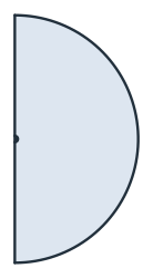
(a) The half plane, 80 radii out

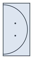
(b) The windings and the air near them

Figure 1: The coil pair in the half plane through its axis

The field

The unknown is \(u = A_\varphi / r\), the vector potential around the axis divided by the distance from it. Unlike \(A_\varphi\) itself, it is smooth on the axis, and the flux density follows from it as

\[B_r = -r \frac{\partial u}{\partial z}, \qquad B_z = 2u + r \frac{\partial u}{\partial r}.\]

In weak form, \(\int r^3 \, \nabla u \cdot \nabla v \, dr \, dz = \int \mu_0 J r^2 v \, dr \, dz\) for every test function \(v\), with the current density \(J\) in the windings. The axis needs no boundary condition, and \(u\) = 0 far away:

def field(s, order=5):
    """the mesh, the flux density (B_r, B_z) and u of the pair with the spacing s"""
    mesh = ngs.Mesh(px.OCCGeometry(pair(s)).GenerateMesh(maxh=80 * R / 6))
    mesh.Curve(order)
    V = ngs.H1(mesh, order=order, dirichlet="far")
    trial, test = V.TnT()
    r = ngs.x
    a = ngs.BilinearForm(r**3 * ngs.grad(trial) * ngs.grad(test) * ngs.dx).Assemble()
    f = ngs.LinearForm(mu0 * J * r**2 * test * ngs.dx("winding")).Assemble()
    u = ngs.GridFunction(V)
    u.vec.data = a.mat.Inverse(V.FreeDofs(), inverse="sparsecholesky") * f.vec
    return mesh, ngs.CF((-r * ngs.grad(u)[1], 2 * u + r * ngs.grad(u)[0])), u


mesh, B, u = field(R)
print(mesh.ne, "triangles | field at the center", B(mesh(0, 0))[1], "T")

22502 triangles | field at the center 0.0005994050118049382 T

The formula for \(B_0\) holds for thin loops. On the axis, one loop of radius \(a\) at the height \(h\) gives the field \(\mu_0 I a^2 / 2 \left(a^2 + (z - h)^2\right)^{3/2}\), and the field of a winding with a section is this loop field summed over the section with SciPy’s dblquad. The computed field at the center lies within a few millionths of it, and the windings’ section moves it from the thin-loop formula by less than a ten-thousandth:

def on_axis(z, s):
    """the field on the axis at the height z, from the loop formula summed over the sections of both windings"""
    def loop(a, h):
        return mu0 * J * a**2 / (2 * (a**2 + (z - h) ** 2) ** 1.5)
    return sum(dblquad(loop, h - c / 2, h + c / 2, R - c / 2, R + c / 2, epsabs=1e-16, epsrel=1e-13)[0]
               for h in (-s / 2, s / 2))


computed, windings, thin = B(mesh(0, 0))[1], on_axis(0, R), (4 / 5) ** 1.5 * mu0 * turns * I / R
print("center: computed", computed, "| windings", windings, "| thin loops", thin)
print("computed / windings - 1", computed / windings - 1, "| windings / thin loops - 1", windings / thin - 1)

center: computed 0.0005994050118049382 | windings 0.0005994066489380157 | thin loops 0.0005994508570488087
computed / windings - 1 -2.731256118604364e-06 | windings / thin loops - 1 -7.374768135404164e-05

The spacing

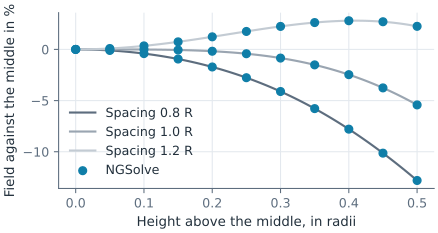
Along the axis, a spacing of 0.8 radii gives a field that is strongest in the middle, 1.2 radii one that is weakest there, and one radius a field that stays flat the longest. Its drop at a tenth of the radius from the middle is close to the fourth-order term of thin loops, \(144/125 \times 10^{-4}\) (Figure 2):

heights = np.linspace(0, 0.5 * R, 11)
profiles, solved = {}, {}
for spacing in (0.8, 1.0, 1.2):
    mesh, B, u = field(spacing * R)
    computed = np.array([B(mesh(0, z))[1] for z in heights])
    exact = np.array([on_axis(z, spacing * R) for z in heights])
    profiles[spacing] = (computed / computed[0] - 1, exact / exact[0] - 1)
    solved[spacing] = (mesh, B, computed[0])
    print("spacing", spacing, "R | at 0.1 R:", profiles[spacing][0][2], "| exact", profiles[spacing][1][2],
          "| at 0.3 R:", profiles[spacing][0][6], "| exact", profiles[spacing][1][6])
print("fourth-order term at 0.1 R", -144 / 125 * 0.1**4)
# plt.plot(heights / R, 100 * profiles[1.0][0]); plt.show()
# px.PlotField(ngs.Norm(B), mesh, pair(1.2 * R))

spacing 0.8 R | at 0.1 R: -0.004087204046147597 | exact -0.0040871936753591465 | at 0.3 R: -0.041121992749418856 | exact -0.041121891911272135
spacing 1.0 R | at 0.1 R: -0.00011744449687378644 | exact -0.00011744358757059814 | at 0.3 R: -0.008464115203944966 | exact -0.008464091625074777
spacing 1.2 R | at 0.1 R: 0.003439023766354854 | exact 0.0034390136857407327 | at 0.3 R: 0.022468304338888467 | exact 0.022468235036374296
fourth-order term at 0.1 R -0.00011520000000000001

Figure 2: The field along the axis for three spacings, the lines from the loop formula

Away from the axis, the field is uniform in a region around the middle that is largest at the Helmholtz spacing. Mirrored about the axis, the plane through the coils shows where the field lies within 2 % of its value in the middle (Figure 3).

(a) Spacing 0.8 R

(b) Spacing 1.0 R

(c) Spacing 1.2 R

Figure 3: The field strength against the middle's, between 0.98 and 1.02

See Identifications for rotational symmetry with periodic edges, and The Halbach array for a field made uniform on one side by the magnets’ layout.