A photonic crystal

Why does a lattice of glass-like rods stop light of some colors? In a photonic crystal, the dielectric constant repeats on the scale of the wavelength, and light in it travels as Bloch waves, \(E(\mathbf{x} + \mathbf{a}) = e^{i \mathbf{k} \cdot \mathbf{a}} E(\mathbf{x})\) for every lattice vector \(\mathbf{a}\). Their frequencies form bands, and between two bands there can be a gap: frequencies at which no light travels through the crystal in any direction. For a square lattice of alumina rods, \(\varepsilon = 8.9\) with the radius \(r = 0.2a\) in air, Joannopoulos, Johnson, Winn and Meade find a gap for the TM modes, with the electric field along the rods, between the first and the second band, with a gap–midgap ratio of 31.4 %.

Here, one unit cell of the crystal is drawn with its opposite sides identified, NGSolve finds the Bloch modes along the edge of the Brillouin zone, and the gap is checked against theirs.

import cmath
import math

import ngsolve as ngs
import numpy as np
import planex as px

The unit cell

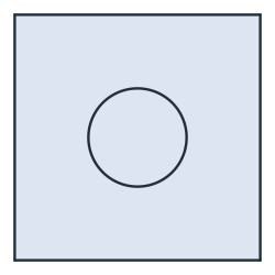
The cell is a square of side \(a = 1\) with the rod in its middle. Its sides are named while drawing, and the rod and the air are glued into one shape with their own names. Identify pairs the left side with the right and the bottom with the top, so netgen meshes them alike (Figure 1). NGSolve takes the Bloch phases in the order of netgen’s numbers for the identifications, and netgen numbers them in the order of the edges, not of the Identify calls. The cell is drawn from its left side, so the left–right pair is number 0:

s = px.QuickSketch((-0.5, 0.5)).Turn(-90).Line(1, name="left").Turn(90).Line(1, name="bottom").Turn(90).Line(1, name="right")
cell = s.Turn(90).Close(name="top").Face()
cell.name = "air"
rod = px.Circle((0, 0), 0.2).Face()
rod.name = "rod"
crystal = px.Glue([cell, rod])
crystal.Identify("left", "right")
crystal.Identify("bottom", "top")
mesh = ngs.Mesh(px.OCCGeometry(crystal).GenerateMesh(maxh=0.05))
mesh.Curve(3)
for number in (0, 1):
    a, b = next(pair for pair, n in mesh.GetPeriodicNodePairs(ngs.VERTEX) if n == number)
    (x0, y0), (x1, y1) = mesh.vertices[a].point, mesh.vertices[b].point
    print("identification", number, "shifts by", (round(x1 - x0, 9), round(y1 - y0, 9)))

identification 0 shifts by (1.0, 0.0)
identification 1 shifts by (0.0, 1.0)

Figure 1: One cell of the square lattice

The Bloch modes

The TM field \(E\) along the rods satisfies \(\nabla^2 E + \varepsilon (\omega/c)^2 E = 0\). NGSolve’s Periodic space joins the identified sides with the Bloch phases \(e^{i k_x}\) and \(e^{i k_y}\), and its ArnoldiSolver finds the eigenvalues \((\omega/c)^2\) nearest a shift. bands asks it for 16 near zero and keeps the lowest four, as the frequencies \(\omega a / (2\pi c)\) for a wave vector \((k_x, k_y)\). Asked for only a few more than are kept, it can miss one of two equal frequencies at \(\Gamma\) and M:

eps = mesh.MaterialCF({"rod": 8.9}, default=1.0)


def bands(kx, ky):
    V = ngs.Periodic(ngs.H1(mesh, order=4, complex=True), phase=[cmath.exp(1j * kx), cmath.exp(1j * ky)])
    u, v = V.TnT()
    a = ngs.BilinearForm(ngs.grad(u) * ngs.grad(v) * ngs.dx).Assemble()
    m = ngs.BilinearForm(eps * u * v * ngs.dx).Assemble()
    modes = ngs.GridFunction(V, multidim=16)
    values = list(ngs.ArnoldiSolver(a.mat, m.mat, V.FreeDofs(), list(modes.vecs), shift=0.01))
    lowest = sorted(range(16), key=lambda k: values[k].real)[:4]
    return [math.sqrt(max(values[k].real, 0)) / (2 * math.pi) for k in lowest], [modes.MDComponent(k) for k in lowest]

The band structure

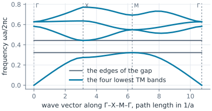
The bands are followed along the edge of the irreducible Brillouin zone, from \(\Gamma\) at \(\mathbf{k} = 0\) to X at \((\pi, 0)\), M at \((\pi, \pi)\) and back to \(\Gamma\), where the lowest and highest frequencies of a band lie in most crystals. The first band never reaches the second, and the gap between them is 31.4 % of its middle (Figure 2):

path = [(t * math.pi, 0) for t in np.linspace(0, 1, 9)] + [(math.pi, t * math.pi) for t in np.linspace(0, 1, 9)[1:]] \
    + [(t * math.pi, t * math.pi) for t in np.linspace(1, 0, 13)[1:]]
diagram = [bands(kx, ky)[0] for kx, ky in path]
first, second = max(b[0] for b in diagram), min(b[1] for b in diagram)
print("first band up to", round(first, 4), "| second band from", round(second, 4))
print("gap-midgap", round((second - first) / ((second + first) / 2), 4), "| Joannopoulos et al. 0.314")

first band up to 0.3224 | second band from 0.4425
gap-midgap 0.3141 | Joannopoulos et al. 0.314

Figure 2: The TM bands of a square lattice of rods, ε = 8.9, r = 0.2a

The two bands at X

At X, the first band’s field gathers in the rods, where the dielectric constant is high and the frequency low. The second band must change sign across each rod to stay orthogonal to the first, so it pushes its field into the air, and its frequency is higher. The second band’s lowest frequency, the upper edge of the gap, lies at X, and the first band’s highest, the lower edge, at M (Figure 3):

frequencies, modes = bands(math.pi, 0)
print("at X:", [round(f, 4) for f in frequencies[:2]])

at X: [0.2747, 0.4425]

(a) Band 1, in the rods

(b) Band 2, in the air

Figure 3: The first two TM modes at X