The Faraday cage

How well does a cage of wires shield its inside from an electric field? The wires of a Faraday cage are conductors at one common potential, and the charges on them cancel most of the outside field inside the cage. The Feynman Lectures derive a field that decays exponentially with the distance from a plane grid of charged wires, and the shielding of a cage is often taken to grow exponentially as the wires get closer together. Chapman, Hewett and Trefethen showed that for a ring of \(n\) round wires of radius \(r\), it does not. The field inside falls only in proportion to \(\log(1/r)/n\).

The example follows their model in 2D. The wires stand on the unit circle, conducting, at one potential and with no net charge. The outside field comes from a line charge at the distance 2 from the center, whose field at the center is \(\tfrac{1}{2}\) without the cage. The field at the center must agree with the values in their paper, and with their homogenized formula where the wires are thin compared to the gaps between them.

import math

import ngsolve as ngs
import planex as px

The cage

The domain is a disc of radius 100 with a hole for each wire. px.Unify joins the wires into one shape, and one subtraction cuts them all out. The wires’ edges are named wire and get a mesh size of half the wire’s radius, and the disc’s edge, far, stands for the far field:

def cage(n, r, far=100):
    """a disc of radius far with n wires of radius r on the unit circle cut out"""
    disc = px.Circle((0, 0), far).Face()
    disc.edges.name = "far"
    wires = [px.Circle((math.cos(2 * math.pi * k / n), math.sin(2 * math.pi * k / n)), r).Face() for k in range(n)]
    for wire in wires:
        wire.edges.name = "wire"
        wire.edges.maxh = r / 2
    return disc - px.Unify(wires)


print("twelve wires of radius 0.01 | area", cage(12, 0.01).mass, "exact", math.pi * (100**2 - 12 * 0.01**2))

twelve wires of radius 0.01 | area 31415.92276598676 exact 31415.922765986747

The potential

The line charge at \(z_s = 2\) has the potential \(\log|z - z_s|\). The cage adds a potential \(\psi\) that is harmonic in the domain, vanishes far away and makes \(\varphi = \log|z - z_s| + \psi\) the same constant \(\varphi_0\) on every wire. \(\varphi_0\) is unknown, and it follows from the condition that the wires carry no net charge. field solves for \(\psi\) twice, once with \(\psi = -\log|z - z_s|\) on the wires and once with \(\psi = 1\) there, both 0 on the far edge. Their combination \(\psi_1 + \varphi_0 \psi_2\) carries no charge on the wires when \(\varphi_0 = -\int \nabla\psi_1 \cdot \nabla\psi_2 \,dA \Big/ \int \nabla\psi_2 \cdot \nabla\psi_2 \,dA\), since the flux of \(\psi\) through the wires equals \(\int \nabla\psi \cdot \nabla\psi_2 \,dA\). The line charge’s own field at the center is \((-\tfrac{1}{2}, 0)\), and field adds the cage’s to it:

def field(n, r):
    """the potential of a cage of n wires of radius r, its mesh and the field strength at the center"""
    mesh = ngs.Mesh(px.OCCGeometry(cage(n, r)).GenerateMesh(maxh=10))
    mesh.Curve(4)
    fes = ngs.H1(mesh, order=4, dirichlet="wire|far")
    u, v = fes.TnT()
    a = ngs.BilinearForm(ngs.grad(u) * ngs.grad(v) * ngs.dx).Assemble()
    inverse = a.mat.Inverse(fes.FreeDofs(), inverse="sparsecholesky")
    charge = ngs.log(ngs.sqrt((ngs.x - 2) ** 2 + ngs.y**2))

    def solve(on_wires):
        psi = ngs.GridFunction(fes)
        psi.Set(on_wires, definedon=mesh.Boundaries("wire"))
        rest = psi.vec.CreateVector()
        rest.data = -a.mat * psi.vec
        psi.vec.data += inverse * rest
        return psi

    psi1, psi2 = solve(-charge), solve(1)
    phi0 = -ngs.Integrate(ngs.grad(psi1) * ngs.grad(psi2), mesh) / ngs.Integrate(ngs.grad(psi2) * ngs.grad(psi2), mesh)
    psi = ngs.GridFunction(fes)
    psi.vec.data = psi1.vec + phi0 * psi2.vec
    gx, gy = ngs.grad(psi)(mesh(0, 0))
    return charge + psi, mesh, math.hypot(gx - 1 / 2, gy)

Twelve wires of radius 0.1, 0.01 and 0.001, as in the paper’s first figure, let more of the field in the thinner they are. The lines are lines of equal potential:

Against the paper

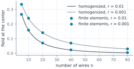
Chapman, Hewett and Trefethen computed the field at the center for this setup with a series solution and list it for \(n\) from 5 to 320 wires and \(r\) from 0.1 to 10⁻⁶. Their homogenized model replaces the wires by a boundary condition on the unit circle and gives the field at the center as \(1/\bigl(|z_s|\,(1 + n/(2 \log(1/(rn))))\bigr)\), for \(rn < 1\). The field at the center for 5 to 80 wires of radius 0.01 and 0.001 is compared with the paper’s table and the homogenized formula:

paper = {0.01: [0.2663, 0.1582, 0.0699, 0.0229, 0.0047], 0.001: [0.3348, 0.2399, 0.1406, 0.0693, 0.0297]}
counts = [5, 10, 20, 40, 80]
fields = {}
for r, table in paper.items():
    fields[r] = [field(n, r)[2] for n in counts]
    for n, strength, value in zip(counts, fields[r], table):
        homogenized = 1 / (2 * (1 + n / (2 * math.log(1 / (r * n)))))
        print("r", r, "| n", n, "| field", round(strength, 5), "| paper", value, "| homogenized", round(homogenized, 4))

r 0.01 | n 5 | field 0.26635 | paper 0.2663 | homogenized 0.2726
r 0.01 | n 10 | field 0.15826 | paper 0.1582 | homogenized 0.1577
r 0.01 | n 20 | field 0.06991 | paper 0.0699 | homogenized 0.0693
r 0.01 | n 40 | field 0.0229 | paper 0.0229 | homogenized 0.0219
r 0.01 | n 80 | field 0.00466 | paper 0.0047 | homogenized 0.0028
r 0.001 | n 5 | field 0.33485 | paper 0.3348 | homogenized 0.3397
r 0.001 | n 10 | field 0.23993 | paper 0.2399 | homogenized 0.2397
r 0.001 | n 20 | field 0.14069 | paper 0.1406 | homogenized 0.1406
r 0.001 | n 40 | field 0.06935 | paper 0.0693 | homogenized 0.0693
r 0.001 | n 80 | field 0.02972 | paper 0.0297 | homogenized 0.0297

The finite elements reproduce the paper’s values to all four of its digits. The homogenized formula comes within about 5 % of them until the gaps between the wires shrink to a few wire diameters, at 80 wires of radius 0.01.

Linear, not exponential

For many thin wires, the homogenized formula is about \(2 \log(1/(rn))/(n\,|z_s|)\), so the field inside falls in proportion to \(1/n\), with a slowly changing logarithm. For wires of radius 0.001, each doubling of the number of wires divides the field at the center by a factor from 1.4 to 2.3, where an exponential decay would square the shielding factor with each doubling. Only where the gaps close up, as for many wires of radius 0.01, does the field drop faster (Figure 1):

Figure 1: The field at the center of the cage, 1/2 without it

See Many faces at once for px.Unify and Meshing a face for meshes with named boundaries.