Section properties of steel profiles

How stiff is a beam’s cross-section? In bending, a beam’s stiffness is \(EI\), the material’s modulus times the second moment of area of its section, \(I = \int y^2\,dA\) about the axis through the section’s centroid. Steel catalogs list \(I\) for every rolled profile, with the elastic section modulus \(W = I / y_{max}\), which gives the bending stress at the outer fiber, and the radius of gyration \(i = \sqrt{I/A}\), which enters the buckling of columns. All of them follow from the profile’s drawing alone. Here they are measured on the drawing and checked against the formulas and the catalogs.

face.Measure() returns them in one dictionary, from the face’s exact lines and arcs:

Key	Value
"area"	The area \(A\)
"center"	The centroid
"Ih", "Iv"	The second moments \(I_h = \int v^2\,dA\) and \(I_v = \int h^2\,dA\) about the horizontal and the vertical axis through the centroid
"Ihv"	The product of inertia \(I_{hv} = \int h v\,dA\)
"I1", "I2", "principal_angle"	The principal moments, the largest and the smallest second moment about an axis through the centroid, and the angle of the axis of \(I_1\) from \(h\) in degrees

import math

import matplotlib.pyplot as plt
import numpy as np
import planex as px

Shapes from the list

The list of second moments of area starts with the simple shapes. The example measures four of them about their centroids (Figure 1):

• a rectangle of 40 × 60, with \(I = bh^3/12\);

• a tube of 60 outside and 50 inside, with \(I = \pi (D^4 - d^4)/64\);

• a half disc of radius 20, with \(I = (\pi/8 - 8/(9\pi))\,r^4\) about its centroid, which lies \(4r/(3\pi)\) above the diameter;

• a right triangle of 30 × 45, with \(I = bh^3/36\).

shapes = {
    "rectangle": (px.QuickSketch().RectangleC(40, 60).Face(), 40 * 60**3 / 12),
    "tube": (px.Circle((0, 0), 30).Face() - px.Circle((0, 0), 25).Face(), math.pi * (60**4 - 50**4) / 64),
    "half disc": (px.QuickSketch((-20, 0)).Line(40).Turn(90).Arc(20, 180).Face(),
                  (math.pi / 8 - 8 / (9 * math.pi)) * 20**4),
    "triangle": (px.QuickSketch().Line(30).Line((0, 45)).Close().Face(), 30 * 45**3 / 36),
}
for name, (face, exact) in shapes.items():
    print(name, "Ih", face.Measure()["Ih"], "exact", exact)
print("half disc centroid", shapes["half disc"][0].Measure()["center"][1], "exact", 4 * 20 / (3 * math.pi))

rectangle Ih 720000.0 exact 720000.0
tube Ih 329376.3547748048 exact 329376.35477480484
half disc Ih 17561.11370343452 exact 17561.113703434516
triangle Ih 75937.5 exact 75937.5
half disc centroid 8.48826363156775 exact 8.48826363156775

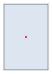
(a) Rectangle

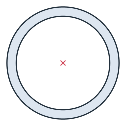
(b) Tube

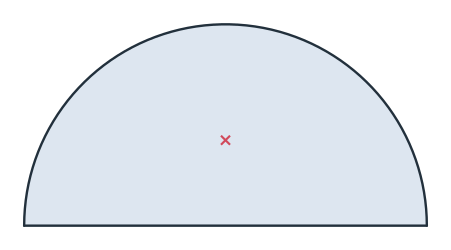
(c) Half disc

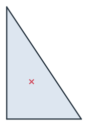
(d) Triangle

Figure 1: Four shapes from the list, their centroids marked

The parallel axis theorem

A built-up section adds the second moments of its parts, each moved to the common axis by the parallel axis theorem, \(I = \sum_i (I_i + A_i d_i^2)\), with \(d_i\) the distance of the part’s centroid from the axis. The example is an IPE 200 without its root radii, a web of 5.6 × 200 and two flanges of 100 × 8.5, united into one face. The theorem takes the web between the flanges, 183 high, and the two flanges at \(d = 100 - 8.5/2\) from the axis:

web = px.QuickSketch().RectangleC(5.6, 200).Face()
flanges = [px.QuickSketch((0, s * (100 - 8.5 / 2))).RectangleC(100, 8.5).Face() for s in (-1, 1)]
sharp = px.Unify([web, *flanges]).Face()
d = 100 - 8.5 / 2
print("Ih", sharp.Measure()["Ih"], "theorem", 5.6 * 183**3 / 12 + 2 * (100 * 8.5**3 / 12 + 100 * 8.5 * d**2))

Ih 18455902.266666654 theorem 18455902.266666666

An IPE 200 against the table

A rolled IPE 200 has root radii of 12 between the web and the flanges. Filleted there, the section has the values of the producers’ tables, for example Stad’s. The tables’ \(y\) axis is the strong axis, horizontal here, so \(I_y\) is "Ih" and \(I_z\) is "Iv". The section moduli divide by the distance of the outer fiber, 100 from the strong axis and 50 from the weak one (Figure 2):

ipe = sharp.Filleted([(s * 5.6 / 2, t * (100 - 8.5)) for s in (-1, 1) for t in (-1, 1)], 12)
m = ipe.Measure()
A = m["area"]
print("A", round(A / 100, 2), "cm², table 28.48")
print("Iy", round(m["Ih"] / 1e4, 1), "cm⁴, table 1943 | Wel,y", round(m["Ih"] / 100 / 1e3, 1), "cm³, table 194.3")
print("iy", round(math.sqrt(m["Ih"] / A) / 10, 2), "cm, table 8.26")
print("Iz", round(m["Iv"] / 1e4, 1), "cm⁴, table 142 | Wel,z", round(m["Iv"] / 50 / 1e3, 1), "cm³, table 28.5")
print("iz", round(math.sqrt(m["Iv"] / A) / 10, 2), "cm, table 2.24")

A 28.48 cm², table 28.48
Iy 1943.2 cm⁴, table 1943 | Wel,y 194.3 cm³, table 194.3
iy 8.26 cm, table 8.26
Iz 142.4 cm⁴, table 142 | Wel,z 28.5 cm³, table 28.5
iz 2.24 cm, table 2.24

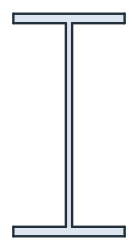
(a) Without the root radii

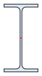
(b) IPE 200, the centroid marked

Figure 2: The IPE 200 from three rectangles, then filleted

The principal axes of an angle

An unequal angle has no axis of symmetry, so its strong axis is tilted. The example is an L 150 × 100 × 10, the long leg upright, with a root radius of 12 inside the corner and toe radii of 6 at the ends of the legs. Drawn with the pen and filleted at its three corners, it has the values of the section table, here as RoyMech lists them. They are the second moments and the product of inertia about the centroid, and the principal moments \(I_1\) and \(I_2\), which the table calls \(I_u\) and \(I_v\), with \(\tan\alpha\) of the axis of \(I_1\) (Figure 3):

angle = px.QuickSketch().Line(100).Turn(90).Line(10).Turn(90).Line(90).Turn(-90).Line(140).Turn(90).Line(10).Close()
profile = angle.Face().Filleted((10, 10), 12).Filleted([(100, 10), (10, 150)], 6)
m = profile.Measure()
print("A", round(m["area"] / 100, 2), "cm², table 24.2")
print("centroid", [round(c / 10, 2) for c in m["center"][:2]], "cm, table 2.34 and 4.81")
print("Ih", round(m["Ih"] / 1e4, 1), "| Iv", round(m["Iv"] / 1e4, 1), "| Ihv", round(m["Ihv"] / 1e4, 1),
      "cm⁴, table 553, 198, -192")
print("I1", round(m["I1"] / 1e4, 1), "| I2", round(m["I2"] / 1e4, 1), "cm⁴, table 637, 114")
print("tan α", round(math.tan(math.radians(m["principal_angle"])), 3), "table 0.438")

A 24.15 cm², table 24.2
centroid [2.34, 4.81] cm, table 2.34 and 4.81
Ih 552.6 | Iv 198.5 | Ihv -192.2 cm⁴, table 553, 198, -192
I1 636.9 | I2 114.2 cm⁴, table 637, 114
tan α 0.438 table 0.438

Figure 3: The unequal angle L 150 × 100 × 10

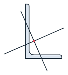
The principal values follow from \(I_h\), \(I_v\) and \(I_{hv}\) by Mohr’s circle. It is centered at \((I_h + I_v)/2\) with the radius \(\sqrt{((I_h - I_v)/2)^2 + I_{hv}^2}\), and the principal axis turns from \(h\) by \(\alpha\) with \(\tan 2\alpha = -2 I_{hv} / (I_h - I_v)\):

c, R = (m["Ih"] + m["Iv"]) / 2, math.hypot((m["Ih"] - m["Iv"]) / 2, m["Ihv"])
print("I1", round((c + R) / 1e4, 1), "| I2", round((c - R) / 1e4, 1), "cm⁴")
print("α", math.degrees(math.atan2(-2 * m["Ihv"], m["Ih"] - m["Iv"])) / 2, "measured", m["principal_angle"])

I1 636.9 | I2 114.2 cm⁴
α 23.675041917497747 measured 23.67504191749775

The circle carries the two points \((I_h, I_{hv})\) and \((I_v, -I_{hv})\) in blue, and the principal moments, red, lie where it crosses the axis: