Open and closed sections in torsion

Why does a slit tube twist so much more easily than a closed one? A thin tube slit along its length keeps almost all of its material but loses almost all of its torsional stiffness. In the closed tube, the shear stress runs around the wall as one shear flow, and Bredt’s formula gives the torsion constant \(J \approx 2\pi R^3 t\), for the mean radius \(R\) and the wall thickness \(t\). In the slit tube, the stress runs along one face of the wall and back along the other, and \(J \approx s t^3/3\), for the length \(s\) of the wall’s midline. The closed tube is about \(3(R/t)^2\) times as stiff, which is why closed box sections carry torsion in frames and bridges, and why a slit tube can serve as a flexure hinge that twists easily.

The example solves Saint-Venant torsion for a tube with a mean radius of 25 and walls of 5, 2.5 and 1.25, closed and slit. The closed tube’s \(J\) must equal \(\pi (R_o^4 - R_i^4)/2\) exactly, the slit tube’s must approach the thin-walled value, and the ratios of their stiffness and of their largest shear stress must approach \(3(R/t)^2\) and \(3R/t\).

import math

import ngsolve as ngs
import planex as px
import planex.measurements as pm

The sections

A tube is a disc less a smaller disc, and the slit tube is the same tube less a rectangle across its wall, as wide as the wall is thick (Figure 1):

R = 25  # the mean radius


def tube(t, slit=False):
    """the section of a tube of wall thickness t, closed or slit along its length"""
    section = px.Circle((0, 0), R + t / 2).Face() - px.Circle((0, 0), R - t / 2).Face()
    if slit:
        section = section - px.QuickSketch((R - t, -t / 2)).Rectangle(2 * t, t).Face()
    return section


print("closed", tube(2.5).mass, "| slit", tube(2.5, slit=True).mass, "| the slit keeps", tube(2.5, True).mass / tube(2.5).mass)

closed 392.69908169872406 | slit 386.4464680466499 | the slit keeps 0.9840778500804565

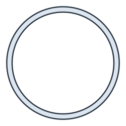
(a) Closed

(b) Slit

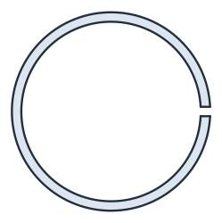
Figure 1: A tube with a wall of 2.5, closed and slit

The torsion constant

pm.TorsionConstant() solves for the warping function of a section, the axial displacement of its points per unit of twist, and integrates \(J\) from it, holes included. The circular tube is the one hollow section that does not warp, and its \(J\) is exactly \(\pi (R_o^4 - R_i^4)/2\), where Bredt’s formula \(4A^2 t/s\), for the area \(A\) inside the midline, gives \(2\pi R^3 t\). The slit tube’s \(J\) is that of a thin curved strip of length \(s = 2\pi R - t\), \(s t^3/3\), less the share of its two ends, which a thin rectangle has as the factor \(1 - 0.630\,t/s\). Both are compared with these values, and their ratio with \(3(R/t)^2\):

J = {}
for t in (5, 2.5, 1.25):
    J[t] = tube(t).Measure(pm.TorsionConstant()), tube(t, slit=True).Measure(pm.TorsionConstant())
    s = 2 * math.pi * R - t
    print("t", t, "| closed", round(J[t][0], 1), "exact", round(math.pi / 2 * ((R + t / 2) ** 4 - (R - t / 2) ** 4), 1),
          "Bredt", round(2 * math.pi * R**3 * t, 1))
    print("     | slit", round(J[t][1], 2), "thin-walled", round(s * t**3 / 3 * (1 - 0.630 * t / s), 2),
          "| ratio", round(J[t][0] / J[t][1], 1), "3(R/t)²", 3 * (R / t) ** 2)

t 5 | closed 495782.6 exact 495782.6 Bredt 490873.9
     | slit 6208.4 thin-walled 6205.4 | ratio 79.9 3(R/t)² 75.0
t 2.5 | closed 246050.5 exact 246050.5 Bredt 245436.9
     | slit 797.22 thin-walled 796.9 | ratio 308.6 3(R/t)² 300.0
t 1.25 | closed 122795.2 exact 122795.2 Bredt 122718.5
     | slit 100.98 thin-walled 100.94 | ratio 1216.0 3(R/t)² 1200.0

The thinner the wall, the closer the ratio comes to \(3(R/t)^2\). At a wall of a twentieth of the radius, the closed tube is over a thousand times as stiff as the slit one.

The shear stress

The shear stress follows from the warping function \(\omega\) as \(\tau = G\theta\,(\partial\omega/\partial x - y, \partial\omega/\partial y + x)\), about the section’s centroid, where \(\theta\) is the twist per unit length. Under a torque \(T\), \(G\theta = T/J\). shear solves Laplace’s equation for \(\omega\) with the boundary condition \(\partial\omega/\partial n = y\,n_x - x\,n_y\) on every edge, as pm.TorsionConstant does, and returns the magnitude of \(\tau\) for a unit torque. In the closed tube, the stress is about \(T/(2At)\), almost the same across the wall. In the slit tube, it changes sign across the wall and reaches about \(T t/J\) at its faces, \(3R/t\) times as much. The largest stress in each is printed, and their ratio is compared with \(3R/t\):

def shear(section, t, order=4):
    """the shear stress for a unit torque, its mesh and its largest value"""
    mesh = ngs.Mesh(px.OCCGeometry(section).GenerateMesh(maxh=t / 2))
    mesh.Curve(order)
    area = ngs.Integrate(1, mesh)
    X = ngs.x - ngs.Integrate(ngs.x, mesh) / area
    Y = ngs.y - ngs.Integrate(ngs.y, mesh) / area
    fes = ngs.H1(mesh, order=order)
    u, v = fes.TnT()
    n = ngs.specialcf.normal(2)
    a = ngs.BilinearForm(ngs.grad(u) * ngs.grad(v) * ngs.dx + 1e-10 * u * v * ngs.dx).Assemble()
    f = ngs.LinearForm((Y * n[0] - X * n[1]) * v * ngs.ds).Assemble()
    w = ngs.GridFunction(fes)
    w.vec.data = a.mat.Inverse(fes.FreeDofs(), inverse="sparsecholesky") * f.vec
    dx, dy = ngs.grad(w)
    J = ngs.Integrate(X * X + Y * Y + X * dy - Y * dx, mesh)
    tau = ngs.sqrt((dx - Y) ** 2 + (dy + X) ** 2) / J
    points = mesh.MapToAllElements(ngs.IntegrationRule(ngs.TRIG, 2 * order), mesh.Materials(".*"))
    return tau, mesh, tau(points).flatten().max()


stresses = {}
for t in (5, 2.5, 1.25):
    stresses[t] = shear(tube(t), t), shear(tube(t, slit=True), t)
    closed, slit = stresses[t][0][2], stresses[t][1][2]
    print("t", t, "| closed", closed, "Bredt", 1 / (2 * math.pi * R**2 * t), "| slit", slit,
          "| ratio", round(slit / closed, 2), "3R/t", 3 * R / t)

t 5 | closed 5.544854942238906e-05 Bredt 5.0929581789406506e-05 | slit 0.0008312601085679633 | ratio 14.99 3R/t 15.0
t 2.5 | closed 0.00010666638625140906 Bredt 0.00010185916357881301 | slit 0.0031777411862031414 | ratio 29.79 3R/t 30.0
t 1.25 | closed 0.00020866207116591033 Bredt 0.00020371832715762603 | slit 0.012431885821528635 | ratio 59.58 3R/t 60.0

For the wall of 5, under the same torque and on the same color scale, the closed tube’s stress hardly shows. In the slit tube, the stress runs along the inner face one way and along the outer face the other way, through zero in the middle of the wall:

See Part analysis for pm.TorsionConstant among the other measurements and Field solvers as measurements for measurements that solve a field.