Transition curves

Why does a road or a railway not run from a straight directly into an arc? On the straight, the curvature is zero, and on an arc of radius \(R\) it is \(1/R\). Joined directly, the curvature jumps, and a vehicle at the speed \(v\) feels the sideways acceleration \(v^2/R\) arrive at once. Between the two goes a transition curve, the Euler spiral or clothoid, whose curvature grows in proportion to its length,

\[\kappa(s) = \frac{s}{A^2}, \qquad A^2 = R L,\]

so that it reaches \(1/R\) at its end, after the length \(L\). Over the transition, the tangent turns by \(L/(2R)\), and the arc moves inward by the shift \(p \approx L^2/(24R)\). A vehicle feels its sideways acceleration grow at the constant rate \(v^3/(R L)\), which sets the transition’s length: \(L = v^3/(C R)\) for an accepted rate \(C\).

Here, the clothoid is drawn from SciPy’s Fresnel integrals as a px.Curve, joined into the curve of a road and checked against these relations. The road turns by 40° on an arc of \(R = 300\) m with transitions of \(L = 100\) m.

import math

import numpy as np
import planex as px
from scipy.interpolate import BSpline
from scipy.special import fresnel

The clothoid

With \(s = A\sqrt{\pi}\,z\), the clothoid’s points are the Fresnel integrals, \(x = A\sqrt{\pi}\,C(z)\) and \(y = A\sqrt{\pi}\,S(z)\), which SciPy’s fresnel computes. px.Curve takes the function and fits it as one spline edge:

R, L = 300.0, 100.0
A = math.sqrt(R * L)
scale = A * math.sqrt(math.pi)


def clothoid(s):
    S, C = fresnel(s / scale)
    return (scale * C, scale * S)


spiral = px.Curve(clothoid, (0, L))
end = spiral.edges[0].TangentAt(1.0)
print("length", spiral.mass, "| turned by", math.degrees(math.atan2(end[1], end[0])), "° | L/2R",
      math.degrees(L / (2 * R)), "°")

length 99.99999999977665 | turned by 9.54929790239125 ° | L/2R 9.54929658551372 °

The curvature follows from the spline’s exact B-spline, as on Curvature-continuous blends. It grows in proportion to the length, and at the end it is \(1/R\):

def curvature(edge, n=2001):
    data = edge.bspline
    p, knots = data["degree"], np.asarray(data["knots"])
    curve = BSpline(knots, np.asarray(data["poles"]), p)
    u = np.linspace(knots[p], knots[-p - 1], n)
    d1, d2 = curve.derivative(1)(u), curve.derivative(2)(u)
    speed = np.hypot(d1[:, 0], d1[:, 1])
    kappa = np.abs(d1[:, 0] * d2[:, 1] - d1[:, 1] * d2[:, 0]) / speed**3
    s = np.concatenate([[0], np.cumsum((speed[1:] + speed[:-1]) / 2 * np.diff(u))])
    return s, kappa


s, kappa = curvature(spiral.edges[0].edge)
print("largest difference from s/A²", np.abs(kappa - s / A**2).max(), "| at the end", kappa[-1], "| 1/R", 1 / R)

largest difference from s/A² 5.6836380957561716e-08 | at the end 0.003333390169707521 | 1/R 0.0033333333333333335

The curve of the road

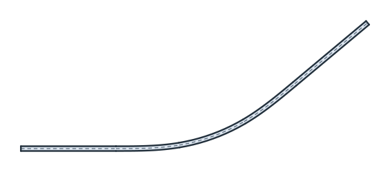
The road comes along a straight of 150 m, runs into the clothoid, turns on the arc and leaves on a second clothoid and a straight. The arc sweeps the 40° less what both transitions turn. The second clothoid is the first one mirrored across the line halfway between the arc’s two ends, run backward, so that it starts where the arc ends. The sketch joins all five into one wire (Figure 1):

sweep = 40 - 2 * math.degrees(L / (2 * R))
road = px.QuickSketch((-150, 0)).Line(150).Curve(clothoid, (0, L)).Arc(R, sweep, id="arc")
start, finish = np.array(clothoid(L)), np.array(road.pen.position)
across = (finish - start) / np.linalg.norm(finish - start)


def mirrored(s):
    p = np.array(clothoid(L - s))
    return tuple(p - 2 * np.dot(p - (start + finish) / 2, across) * across)


road.Curve(mirrored, (0, L)).Line(150)
centerline = road.Wire()
print(len(road.Wires()), "wire | length", centerline.mass, "| exact", 2 * 150 + 2 * L + R * math.radians(sweep))

1 wire | length 609.4395102388729 | exact 609.4395102393196

The road surface is 7.5 m wide, the centerline offset by 3.75 m to each side with flat ends. A band of constant width along a curve has the area of its width times its length, as long as it does not fold, and this one keeps it:

surface = centerline.Offset(3.75, ends=px.Flat)
print("area", surface.mass, "| 7.5 times the length", 7.5 * centerline.mass)

area 4570.796330707488 | 7.5 times the length 4570.796326791547

Figure 1: A road curve of 40°

The shift of the circle

The transitions move the arc inward, away from the straight’s line. The arc’s center lies \(R + p\) from that line, and Measure gives the center. The approximation \(L^2/(24R)\) is good to a tenth of a percent here, and the clothoid’s exact end gives \(p = y(L) - R\,(1 - \cos(L/2R))\):

center = road.Measure("arc")["center"]
y_end = clothoid(L)[1]
print("shift", center[1] - R, "| L²/24R", L**2 / (24 * R), "| exact", y_end - R * (1 - math.cos(L / (2 * R))))

shift 1.3875106906302221 | L²/24R 1.3888888888888888 | exact 1.3875118345063182

The curvature along the road

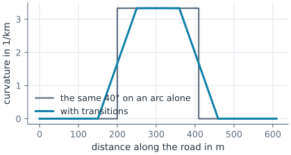
Along the road, the curvature rises from zero on the straight to \(1/R\) on the arc and falls back to zero, a ramp on each clothoid. A road without transitions would jump from zero to \(1/R\) and back (Figure 2):

Figure 2: The curvature along the road

The ride

At 80 km/h, the sideways acceleration on the arc is \(v^2/R\). On the clothoid it grows at the constant rate \(v^3/A^2\) for the \(L/v\) the transition takes. Without the transitions, it arrives at once:

v = 80 / 3.6
print("on the arc", round(v**2 / R, 3), "m/s² | grows at", round(v**3 / A**2, 3), "m/s³ | for", round(L / v, 1), "s")

on the arc 1.646 m/s² | grows at 0.366 m/s³ | for 4.5 s