The Tesla valve

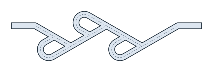
Nikola Tesla’s “valvular conduit” is a channel without moving parts through which a fluid flows more easily one way than the other. Along the channel, buckets branch off at its bends. Flowing one way, the fluid passes their mouths. Flowing the other way, it runs straight into them, around their islands and back into the channel against itself. The ratio of the two pressure drops at the same flow is the valve’s diodicity.

At low speed, the valve does not work at all. Stokes flow is reversible. With the flow reversed at the ends of the channel, it reverses everywhere and costs the same pressure, so the diodicity is exactly 1. Only inertia makes a valve of the channel. The example builds a channel with three buckets from centerlines and offsets, checks the diodicity of 1 in Stokes flow, and follows it with the Navier–Stokes equations up to a Reynolds number of 200.

The speed of the flow from right to left at Re 200, with the buckets carrying it back against the channel

[1]:

import math
import numpy as np
import ngsolve as ngs
from ngsolve.solvers import Newton
import planex as px

The channel

The channel is \(w = 1\) wide. Its centerline is a zigzag of four segments at ±30°, each 6 long in \(x\). At each of the three inner corners, a bucket runs straight on from the segment after the corner, for \(b = 3.5\), turns around an arc of radius \(R = 1.4\) and runs back into the segment before the corner, enclosing an island. bucket draws its centerline as a quick sketch. After the arc, the pen points back toward the channel, and the last line ends where it meets the segment before the corner. Each centerline, offset by \(w/2\) to both sides, is a strip of the channel’s width.

[3]:

w = 1.0
b = 3.5
R = 1.4
rise = 6 * math.tan(math.radians(30))
corners = [(6 * k, rise / 2 if k % 2 == 0 else -rise / 2) for k in range(5)]


def bucket(before, corner, after):
    """the centerline from the corner, straight on from the segment after it, around and into the segment before it"""
    length = math.dist(corner, after)
    d = ((after[0] - corner[0]) / length, (after[1] - corner[1]) / length)
    turn = -180 if corner[1] < 0 else 180  # clockwise below the channel, counterclockwise above
    sketch = px.QuickSketch().Move(corner, dir=(-d[0], -d[1])).Line(b).Arc(R, turn)
    end = sketch.pen.position
    back = px.Line(end, (end[0] + 10 * d[0], end[1] + 10 * d[1]))
    meet = back.Intersections(px.Line(before, corner))[0]
    return sketch.Line((meet.x, meet.y)).Wires()[0]


centerlines = [px.FromPolyline(corners)] + [bucket(*corners[k - 1:k + 2]) for k in (1, 2, 3)]
strips = [line.Offset(w / 2) for line in centerlines]

Straight leads of length 4 at both ends let the flow come in and leave along \(x\). Their ends are named inlet on the left and outlet on the right, so that the mesh knows them. United, the strips and the leads are the valve (Figure 1):

[4]:

x0, y0 = corners[0][0] - 4, corners[0][1] - w / 2
x1, y1 = corners[-1][0], corners[-1][1] - w / 2
left = px.QuickSketch((x0, y0)).Line(4).Turn(90).Line(w).Turn(90).Line(4).Turn(90).Line(w, name="inlet")
right = px.QuickSketch((x1, y1)).Line(4).Turn(90).Line(w, name="outlet").Turn(90).Line(4).Turn(90).Line(w)
valve = px.Unify(strips + [left.Face(), right.Face()]).Face()
print("area", valve.mass, "| named ends", sorted(str(e.name) for e in valve.edges if e.name))

area 61.590583287532525 | named ends ['inlet', 'outlet']

The channel, the centerlines dashed — Figure 1: A Tesla valve of three buckets, from centerlines and offsets

The flow

The mesh comes from the face as it is, with its named ends. Velocity and pressure are Taylor–Hood elements, quadratic and linear. At both ends the velocity is a parabolic profile of mean 1 across the channel, along \(+x\) for the flow from left to right and along \(-x\) for the flow from right to left, and the velocity is zero on the walls. With the velocity given on the whole boundary, the pressure is known only up to a constant, and a Lagrange multiplier sets its mean to 0. In units of the channel’s width and the mean speed, the Reynolds number is \(\mathrm{Re} = 1/\nu\). solve returns the flow and its pressure drop, from the end where the fluid comes in to the end where it leaves. Newton’s method solves the Navier–Stokes equations, starting from a given flow.

[6]:

mesh = ngs.Mesh(px.OCCGeometry(valve).GenerateMesh(maxh=0.15))
mesh.Curve(3)
X = ngs.VectorH1(mesh, order=2, dirichlet=".*") * ngs.H1(mesh, order=1) * ngs.NumberSpace(mesh)
(u, p, lam), (v, q, mu) = X.TnT()
ends = {"inlet": (ngs.y - y0) / w, "outlet": (ngs.y - y1) / w}


def solve(nu, sign, inertia=True, start=None):
    """the flow at the viscosity nu, from left to right (sign 1) or back, and its pressure drop"""
    flow = ngs.GridFunction(X)
    if start is not None:
        flow.vec.data = start.vec
    profile = {name: ngs.CF((sign * 6 * s * (1 - s), 0)) for name, s in ends.items()}
    flow.components[0].Set(mesh.BoundaryCF(profile, default=ngs.CF((0, 0))), definedon=mesh.Boundaries("inlet|outlet"))
    form = nu * ngs.InnerProduct(ngs.grad(u), ngs.grad(v)) - ngs.div(v) * p - ngs.div(u) * q + p * mu + q * lam
    if inertia:
        form += ngs.InnerProduct(ngs.grad(u) * u, v)
    Newton(ngs.BilinearForm(form * ngs.dx), flow, freedofs=X.FreeDofs(), maxerr=1e-10, inverse="umfpack",
           printing=False)
    mean = {name: ngs.Integrate(flow.components[1], mesh, ngs.BND, definedon=mesh.Boundaries(name)) / w
            for name in ends}
    drop = mean["inlet"] - mean["outlet"] if sign > 0 else mean["outlet"] - mean["inlet"]
    return flow, drop


print(mesh.ne, "elements")

5728 elements

Stokes flow is reversible

Without inertia, the equations are linear and have no preferred direction. With the velocity at the ends reversed, the reversed velocity and pressure solve them again, so the pressure drop is the same both ways. The diodicity, the drop from right to left over the drop from left to right, must be 1:

[7]:

stokes = {sign: solve(1.0, sign, inertia=False) for sign in (1, -1)}
forward, backward = stokes[1][1], stokes[-1][1]
print("Stokes: left to right", forward, "right to left", backward, "diodicity", backward / forward)

Stokes: left to right 379.9541814757963 right to left 379.9541814757963 diodicity 1.0

Inertia makes a valve

With inertia, the flow at Re 25 starts from Stokes flow, and each higher Reynolds number from the flow at the one before, so that Newton’s method starts close to the solution:

[8]:

flows = {sign: stokes[sign][0] for sign in (1, -1)}
for Re in (25, 50, 100, 125, 150, 175, 200):
    drops = {}
    for sign in (1, -1):
        flows[sign], drops[sign] = solve(1 / Re, sign, start=flows[sign])
    print("Re", Re, "left to right", drops[1], "right to left", drops[-1], "diodicity", drops[-1] / drops[1])

Re 25 left to right 15.74073700728467 right to left 15.846450035029221 diodicity 1.0067158880613805
Re 50 left to right 8.205081459689033 right to left 8.536510790456115 diodicity 1.040393179811239
Re 100 left to right 4.3877605346454125 right to left 5.191323187698385 diodicity 1.1831373081343217
Re 125 left to right 3.6275472976767915 right to left 4.6442129146217415 diodicity 1.280262539263391
Re 150 left to right 3.1302559058398005 right to left 4.326223821658399 diodicity 1.3820671382130139
Re 175 left to right 2.7862644433927306 right to left 4.126505594683117 diodicity 1.4810172108640285
Re 200 left to right 2.540644455100276 right to left 3.987358623344533 diodicity 1.5694280304904595

From left to right, the flow follows the zigzag and passes the buckets’ mouths. From right to left, it runs straight into the buckets at the corners, around the islands and back into the channel against itself (Figure 2), and the pressure falls more steeply along the way (Figure 3). The flow through the first bucket, measured across it halfway along its straight part, is compared with the flow of 1 through the channel:

[9]:

first = corners[1]
length = math.dist(first, corners[2])
d = ((corners[2][0] - first[0]) / length, (corners[2][1] - first[1]) / length)
across = np.linspace(-w / 2, w / 2, 81)[1:-1]
points = [(first[0] - b / 2 * d[0] - s * d[1], first[1] - b / 2 * d[1] + s * d[0]) for s in across]
xs, ys = np.array(points).T
for sign, name in ((1, "left to right"), (-1, "right to left")):
    velocity = np.asarray(flows[sign].components[0](mesh(xs, ys)))
    into = np.trapezoid(-(velocity[:, 0] * d[0] + velocity[:, 1] * d[1]), across)
    print(name, "| through the first bucket, away from its corner", into)

left to right | through the first bucket, away from its corner -0.031207258330113216
right to left | through the first bucket, away from its corner 0.6016792356609677

(a) Left to right

Right to left — Figure 2: The speed at Re 200, both ways at a mean speed of 1

(a) Left to right

At Re 200 the flow from right to left costs about 1.6 times the pressure of the flow from left to right, with three buckets. Tesla’s drawing has eleven of them, and the diodicity grows with their number and with the speed. See Meshing a face for meshes from planex2d faces.