The golden spiral and the Fibonacci spiral

Is the spiral drawn through the Fibonacci squares the golden spiral? Squares with the Fibonacci numbers 1, 1, 2, 3, 5, 8, … as sides tile a rectangle whose sides approach the golden ratio \(\varphi = (1 + \sqrt{5})/2\), and a quarter circle in each square makes the well-known Fibonacci spiral. The golden spiral is the logarithmic spiral that grows by \(\varphi\) every quarter turn,

\[r = r_0 \, \varphi^{2 \theta / \pi} = r_0 \, e^{b \theta}, \qquad b = \frac{2 \ln \varphi}{\pi}.\]

The two look alike but are different curves. The quarter circles change their curvature at every square, while the logarithmic spiral bends evenly, and even in exactly golden squares the circles stray from it.

The example tiles the Fibonacci squares and checks their area, draws the Fibonacci spiral with arcs and checks its length, draws the golden spiral with px.Curve and checks its length, and measures how far the quarter circles of exactly golden squares run from it.

This page is part of a collection of geometry and design examples using planex2d.

Open this example in the playground, the interactive code editor in the browser, to change the code and run it.

import math

import numpy as np
import planex as px

The Fibonacci squares

Starting from a unit square, each new square is added along the long side of the rectangle so far, in turn on the right, at the top, on the left and at the bottom. The squares tile a rectangle of \(F_n\) by \(F_{n+1}\), so the sum of their areas is \(F_1^2 + \dots + F_n^2 = F_n F_{n+1}\), and the ratio of the sides tends to \(\varphi\) (Figure 1):

phi = (1 + math.sqrt(5)) / 2
F = [1, 1, 2, 3, 5, 8, 13, 21, 34, 55]
x0, y0, x1, y1 = 0, 0, 1, 1
squares = [px.QuickSketch().Rectangle(1, 1).Face()]
for k, s in enumerate(F[1:], 1):
    if k % 4 == 1:
        corner, x1 = (x1, y0), x1 + s
    elif k % 4 == 2:
        corner, y1 = (x0, y1), y1 + s
    elif k % 4 == 3:
        corner, x0 = (x0 - s, y0), x0 - s
    else:
        corner, y0 = (x0, y0 - s), y0 - s
    squares.append(px.QuickSketch().Move(corner).Rectangle(s, s).Face())
tiling = px.Unify(squares)
print("faces", len(tiling.faces), "| area", tiling.mass, "| Σ F²", sum(s * s for s in F), "| F_n F_n+1", 55 * 89)
print("sides", tiling.bounding_box, "| ratio", 89 / 55, "| φ", phi)

faces 1 | area 4895.0 | Σ F² 4895 | F_n F_n+1 4895
sides ((-24.0, -39.0), (65.0, 16.0)) | ratio 1.6181818181818182 | φ 1.618033988749895

The Fibonacci spiral

The spiral is a chain of quarter circles, one in each square with the square’s side as radius. Drawn as a turtle, it starts at (0, 1) heading down and turns left by 90° along each arc. The arcs are exact, so the length is \(\frac{\pi}{2} \sum F_k\) (Figure 1):

pen = px.QuickSketch().Move((0, 1), dir=(0, -1))
for s in F:
    pen = pen.Arc(s, 90)
fibonacci = pen.Wires()[0]
print("length", fibonacci.mass, "| π/2 Σ F", math.pi / 2 * sum(F))
# px.Plot(px.Compound(squares + [fibonacci]))

length 224.62387473167018 | π/2 Σ F 224.6238747316702

Figure 1: The Fibonacci squares and their spiral of quarter circles

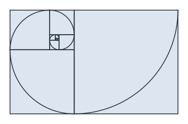
At every joint, the radius jumps from one Fibonacci number to the next, by a factor that tends to \(\varphi\). The golden spiral has no such jumps, since its radius of curvature, \(r \sqrt{1 + b^2}\), grows evenly with \(r\).

The golden spiral

Drawn in exactly golden squares, with the sides \(\varphi^k\), the same chain of quarter circles has its joints on a logarithmic spiral. Each joint is reached from the one before by \(r_k (1 + i) h_k\), as complex numbers with the heading \(h_k\), and these steps shrink by \(\varphi\) and turn back a quarter turn going inward. Their sum to infinity is a geometric series, and it gives the pole the spiral winds into:

radii = [phi**k for k in range(-6, 7)]
start, heading = complex(0, 1), complex(0, -1)
pole = start - radii[0] * (1 + 1j) * heading * (-1j / phi) / (1 + 1j / phi)
pen = px.QuickSketch().Move((0, 1), dir=(0, -1))
joints = [start]
for r in radii:
    pen = pen.Arc(r, 90)
    joints.append(joints[-1] + r * (1 + 1j) * heading)
    heading *= 1j
golden_arcs = pen.Wires()[0]
print("distances of the joints from the pole grow by", [abs(joints[k + 1] - pole) / abs(joints[k] - pole) for k in range(3)])

distances of the joints from the pole grow by [1.6180339887498951, 1.6180339887498953, 1.6180339887498956]

The golden spiral through the first joint is drawn with px.Curve from a Python function. A logarithmic spiral has a finite length from its pole, and between two radii it is \((r_1 - r_0) \sqrt{1 + 1/b^2}\) long:

b = 2 * math.log(phi) / math.pi
r0, theta0 = abs(start - pole), math.atan2((start - pole).imag, (start - pole).real)
turns = len(radii) * math.pi / 2


def golden(t):
    """the golden spiral t radians on from the first joint"""
    r = r0 * math.exp(b * t)
    return (pole.real + r * math.cos(theta0 + t), pole.imag + r * math.sin(theta0 + t))


spiral = px.Curve(golden, (0, turns))
print("length", spiral.mass, "| (r1 - r0) √(1 + 1/b²)", (r0 * math.exp(b * turns) - r0) * math.sqrt(1 + 1 / b**2))

length 73.55635349309526 | (r1 - r0) √(1 + 1/b²) 73.55635350002686

How far apart

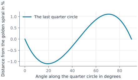
Along the chain of quarter circles, its distance from the pole is compared with the golden spiral’s at the same angle. Between the joints, where they meet the spiral, the circles first run inside it and then outside, by up to about a hundredth of the radius either way. Every quarter circle does the same, and Figure 2 shows the last one:

points = np.array(golden_arcs.Polylines(1e-5)[0])
z = points[:, 0] + 1j * points[:, 1] - pole
theta = np.unwrap(np.angle(z))
deviation = np.abs(z) / (r0 * np.exp(b * (theta - theta[0]))) - 1
print("largest", deviation.max(), "| smallest", deviation.min())
print("Hausdorff distance", golden_arcs.Hausdorff(spiral), "| the largest radius", radii[-1])
# plt.plot((theta - theta[0]) / (math.pi / 2), 100 * deviation); plt.show()

largest 0.011090896617117707 | smallest -0.010969237933565745
Hausdorff distance 0.20716175303185874 | the largest radius 17.944271909999163

Figure 2: How far a quarter circle runs from the golden spiral

See Curves from equations for px.Curve and Sunflower seeds and the golden angle for \(\varphi\) in nature.