Microstrip impedance

How wide must a trace on a circuit board be for a characteristic impedance of 50 Ω? A microstrip is a trace on top of a substrate, with a ground plane below it. Part of its field runs through the substrate and part through the air above, so a signal on it travels as if the whole line were embedded in an effective permittivity \(\varepsilon_{\mathrm{eff}}\) between 1 and the substrate’s \(\varepsilon_r\). Its impedance depends on the ratio of the trace’s width \(W\) to the substrate’s thickness \(h\), and for a thin trace, the closed-form formulas of Hammerstad and Jensen give \(Z_0\) and \(\varepsilon_{\mathrm{eff}}\).

The example computes both from the cross section itself. Two electrostatic solves give the capacitance per length of the line with its substrate and of the same line in air, and from them \(Z_0\) and \(\varepsilon_{\mathrm{eff}}\) follow without any fitted formula. They must agree with Hammerstad and Jensen, and a root search over the width then finds the 50 Ω trace.

import math

import ngsolve as ngs
from scipy.optimize import brentq
import planex as px

The cross section

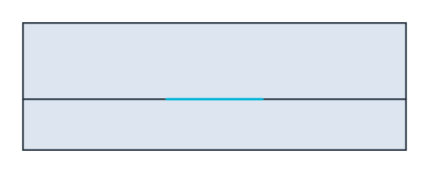
The example is a trace on FR-4, a glass-epoxy laminate, here with \(\varepsilon_r = 4.4\) and \(h = 1.6\,\text{mm}\). The trace is infinitely thin, as in Hammerstad and Jensen’s formulas. The section lies in a box 160 times as wide as the substrate is thick and half as high, whose walls are far enough away to change the result only in the fifth digit, and the box’s bottom is the ground plane. section glues the substrate, the air above it and the trace into one shape. The trace is a line on the interface, which splits the interface’s edge, so the trace has an edge of its own, named trace. The field is singular at the trace’s two edges, so its mesh size is 0.01 mm (Figure 1):

h, er = 1.6, 4.4  # the substrate's thickness in mm and its relative permittivity


def section(W, box=160 * h):
    """the cross section of a trace W wide on the substrate, in a box whose bottom is the ground plane"""
    substrate = px.QuickSketch((-box / 2, 0)).Line(box, 0, name="ground").Line(0, h, name="shield").Line(-box, 0)
    substrate = substrate.Close(name="shield").Face()
    substrate.name = "substrate"
    air = px.QuickSketch((-box / 2, h)).Line(box, 0).Line(0, box / 2 - h, name="shield").Line(-box, 0, name="shield")
    air = air.Close(name="shield").Face()
    air.name = "air"
    trace = px.Line((-W / 2, h), (W / 2, h))
    trace.name = "trace"
    trace.maxh = 0.01
    return px.Glue([substrate, air, trace])


board = section(3)
print("faces", [face.name for face in board.faces], "| boundaries", sorted({e.name for e in board.edges if e.name}))

faces ['substrate', 'air'] | boundaries ['ground', 'shield', 'trace']

Figure 1: The substrate and the air around a trace 3 wide, the trace in cyan

Capacitance per length

The trace is held at 1 V, the ground plane and the box at 0 V. NGSolve solves \(\nabla \cdot (\varepsilon_r \nabla\varphi) = 0\) for the potential \(\varphi\), and the energy of the field gives the capacitance per length, \(C = \varepsilon_0 \int \varepsilon_r\,|\nabla\varphi|^2\,dA\). The same section with air in place of the substrate gives \(C_{\mathrm{air}}\). The line’s effective permittivity is the ratio of the two, \(\varepsilon_{\mathrm{eff}} = C/C_{\mathrm{air}}\), and its characteristic impedance is \(Z_0 = 1/(c\sqrt{C\,C_{\mathrm{air}}})\), with the speed of light \(c\). A cross section has no length, so \(C\) comes out per meter whatever the unit of the drawing:

def line(W, order=5):
    """the characteristic impedance, the effective permittivity and the potential of a trace W wide"""
    mesh = ngs.Mesh(px.OCCGeometry(section(W)).GenerateMesh(maxh=8 * h))
    mesh.Curve(order)
    fes = ngs.H1(mesh, order=order, dirichlet="ground|shield|trace")
    u, v = fes.TnT()
    C, potentials = [], []
    for eps_r in (er, 1):
        eps = mesh.MaterialCF({"substrate": eps_r}, default=1)
        a = ngs.BilinearForm(eps * ngs.grad(u) * ngs.grad(v) * ngs.dx).Assemble()
        phi = ngs.GridFunction(fes)
        phi.Set(1, definedon=mesh.Boundaries("trace"))
        rest = phi.vec.CreateVector()
        rest.data = -a.mat * phi.vec
        phi.vec.data += a.mat.Inverse(fes.FreeDofs(), inverse="sparsecholesky") * rest
        C.append(8.8541878128e-12 * ngs.Integrate(eps * ngs.grad(phi) * ngs.grad(phi), mesh))
        potentials.append(phi)
    return 1 / (299792458 * math.sqrt(C[0] * C[1])), C[0] / C[1], potentials[0], mesh


Z0, eff, phi, mesh = line(3)
print("W 3 mm | Z0", Z0, "ohm | effective permittivity", eff)

W 3 mm | Z0 50.604156311314156 ohm | effective permittivity 3.3254784397174024

Most of the potential falls across the substrate under the trace, and the lines of equal potential crowd at the trace’s edges, where the field is singular:

Against Hammerstad and Jensen

Hammerstad and Jensen fitted closed forms for the impedance and the effective permittivity of an infinitely thin microstrip. With \(u = W/h\), the impedance in air is \(Z_{01} = \eta_0/(2\pi)\,\ln\bigl(f(u)/u + \sqrt{1 + (2/u)^2}\bigr)\), with \(f(u) = 6 + (2\pi - 6)\,e^{-(30.666/u)^{0.7528}}\) and the impedance of free space \(\eta_0\). The effective permittivity is \(\varepsilon_{\mathrm{eff}} = \tfrac{\varepsilon_r + 1}{2} + \tfrac{\varepsilon_r - 1}{2}\,(1 + 10/u)^{-ab}\), with \(a(u)\) and \(b(\varepsilon_r)\) as in hammerstad, and \(Z_0 = Z_{01}/\sqrt{\varepsilon_{\mathrm{eff}}}\). Both are compared for traces from a third of the substrate’s thickness to three times it:

def hammerstad(W):
    """Hammerstad and Jensen's characteristic impedance and effective permittivity of a trace W wide"""
    u = W / h
    a = 1 + math.log((u**4 + (u / 52) ** 2) / (u**4 + 0.432)) / 49 + math.log(1 + (u / 18.1) ** 3) / 18.7
    b = 0.564 * ((er - 0.9) / (er + 3)) ** 0.053
    eff = (er + 1) / 2 + (er - 1) / 2 * (1 + 10 / u) ** (-a * b)
    f = 6 + (2 * math.pi - 6) * math.exp(-((30.666 / u) ** 0.7528))
    z01 = 376.730313668 / (2 * math.pi) * math.log(f / u + math.sqrt(1 + (2 / u) ** 2))
    return z01 / math.sqrt(eff), eff


widths = [0.5, 1, 2, 3, 4, 5]
for W in widths:
    Z0, eff = line(W)[:2]
    z, e = hammerstad(W)
    print("W", W, "mm | Z0", round(Z0, 3), "formula", round(z, 3), "| effective permittivity", round(eff, 5),
          "formula", round(e, 5))

W 0.5 mm | Z0 112.35 formula 112.424 | effective permittivity 2.99821 formula 2.99627
W 1 mm | Z0 87.42 formula 87.481 | effective permittivity 3.08428 formula 3.08172
W 2 mm | Z0 63.484 formula 63.503 | effective permittivity 3.2188 formula 3.21868
W 3 mm | Z0 50.604 formula 50.617 | effective permittivity 3.32548 formula 3.32545
W 4 mm | Z0 42.284 formula 42.308 | effective permittivity 3.4125 formula 3.41056
W 5 mm | Z0 36.407 formula 36.439 | effective permittivity 3.48464 formula 3.48082

The two agree within about 0.1 %, which is within the 0.2 % that Hammerstad and Jensen’s formula is said to hold for the effective permittivity.

A 50 Ω trace

SciPy’s brentq finds the width at which the computed impedance is 50 Ω, between traces of 1 and 5 mm, and the same for the formula:

W50 = brentq(lambda W: line(W)[0] - 50, 1, 5, xtol=1e-5)
W50_formula = brentq(lambda W: hammerstad(W)[0] - 50, 1, 5, xtol=1e-9)
print("50 ohm: W", round(W50, 4), "mm, W/h", round(W50 / h, 4), "| formula: W", round(W50_formula, 4), "mm")

50 ohm: W 3.0607 mm, W/h 1.9129 | formula: W 3.0621 mm

The 50 Ω trace on this board is 3.06 mm wide, 1.9 times the substrate’s thickness, and the formula’s width differs from it by 0.05 %. The rule of thumb that a 50 Ω trace on FR-4 is twice as wide as the substrate is thick holds for \(\varepsilon_r\) of about 4. At the 4.4 taken here, the trace is a little narrower.

See Gluing faces for px.Glue and Meshing a face for meshes with named regions and boundaries.