Simulations
The editor simulates a result of its tree in six ways: a stress analysis in plane stress, the natural frequencies of a plate, heat transfer, electrostatics, magnetics, and the beam calculator, which takes the result as the cross-section of a beam. A simulation is an item of its own in the Simulations section below the tree. It keeps its settings in the project file, and a change of the part marks it out of date until it is solved again. netgen meshes the part and NGSolve solves it in the page, so nothing is uploaded. Lengths are in millimeters.
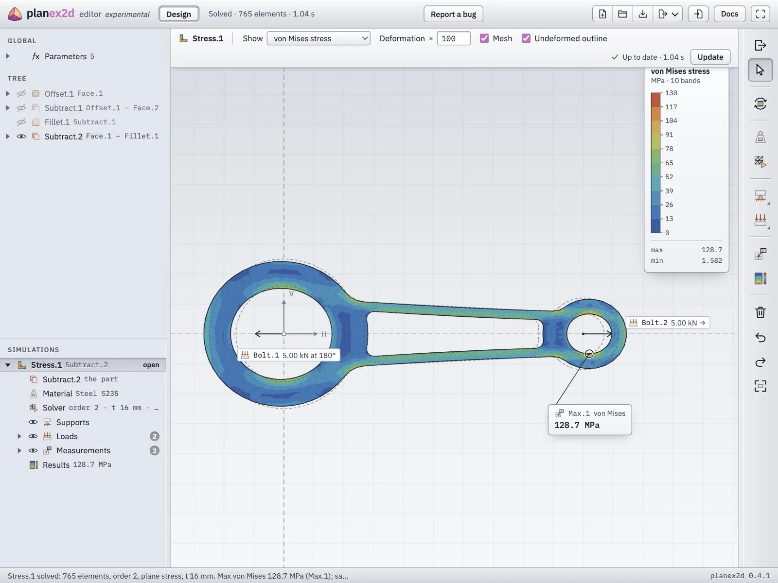
The connecting rod in a stress analysis, pulled at both bores.
Adding a simulation
The six tools of the Simulate group in the Design toolbar add a simulation of their type. Stress analysis is on the button, and the other five open beside it with a right-click, or a long press on a touch screen.
Select the result to simulate, in the tree or in the view.
Click the tool of the simulation type.
The simulation opens in its workbench, named Stress.1, Plate.1, Heat.1, Electro.1, Magnetic.1 or Beam.1.
With nothing selected, the tool asks for the result, which is then clicked in the view or in the tree and taken with OK. A result can have several simulations, of one type or of several, each with its own settings.
The workbench
A simulation is edited in a workbench of its own, the way a sketch is. Its item in the Simulations section folds open to the part, the settings, the supports and loads or the boundary conditions, the measurements and the results, and the toolbar on the right holds one tool for each of them. A click on an item, or on its tool, opens its popup over the view, a table with one row per support, load or region. Exit at the top of the toolbar goes back to Design, and a double-click on the simulation’s item opens the workbench again.
The connecting rod of the tour of the editor is held by the two pins in its bores, so it has no fixed edge. A fixed hole would hold the bore rigidly, which a pin does not.
Select the rod’s last operation, Subtract.2, and click Stress analysis.
Open Solver, set the thickness to 16 mm and tick Balanced holding.
Open Loads and click Add. Choose Bolt load, click the big bore in the view, and type 5000 N at 180°.
Add a second bolt load on the small bore, 5000 N at 0°.
The two loads balance, so balanced holding keeps the part in place without a support, and the results show no unbalanced load.
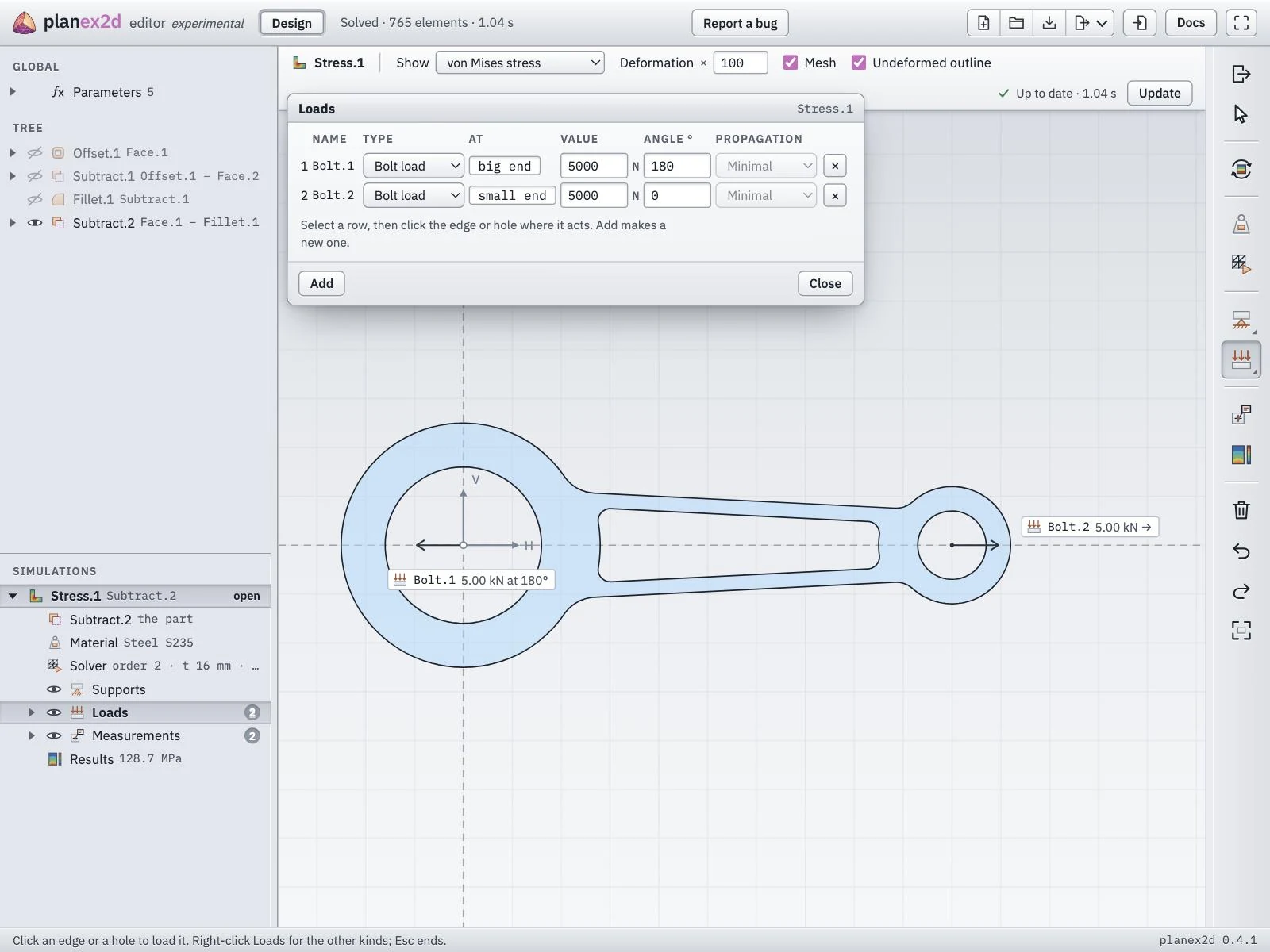
The rod’s two bolt loads, set on the bores named big end and small end.
Places on the part
The At of a row is a place on the part, an edge, a hole or a region, picked with a click in the view. A place takes the name set with Properties, so the rod’s bores are big end and small end. The other edges, holes and regions are numbered by the simulation, E1, E2 and so on for edges, H1 for holes and F1 for regions.
A row stays on its place by name. After a change of the part, a row on a named place stays where it was, while a number can then belong to another edge. Name the places that carry supports and loads.
Propagation continues a row on an edge across its ends, to every edge joined end to end, or only across tangent or curvature-continuous joins. The view marks the whole chain.
The eye in front of a folder or a row shows or hides it in the view.
Solving
Solve in the results bar above the view meshes the part and solves it. The first workbench of a type loads its solver, which takes a few seconds. The mesh follows the mesh sizes set with Properties. A face’s largest element size replaces the simulation’s own default, and an edge’s size refines the mesh along that edge. Simplify outline in the Solver popup, ticked by default, fits arcs to the outline and removes tiny edges before meshing.
The header and the item show the state. A simulation is “Not solved” until its first solve, and a changed setting or a change of the part marks it out of date, with a dot on its item and on Update. A change of the part includes the names and mesh sizes set with Properties. Update solves again with the current settings.
Results in the view
A solved simulation shows its result over the part. The results bar sets what the view shows:
Show chooses the field, such as the von Mises stress, a displacement or the safety factor of a stress analysis.
Deformation scales the deformed shape of a stress analysis, and Undeformed outline draws the part as drawn, dashed.
Mesh draws the mesh lines over the bands.
Field lines in electrostatics and Flux lines in magnetics draw the lines of the field, with their number in the box beside them.
The color scale beside the view gives the bands with their values. Chips in the view name the supports, the loads and the measurements, and a click on one unfolds its row in the tree. A chip can be dragged out of the way.
The Results popup lists the full results, and holds the color scale and its range.
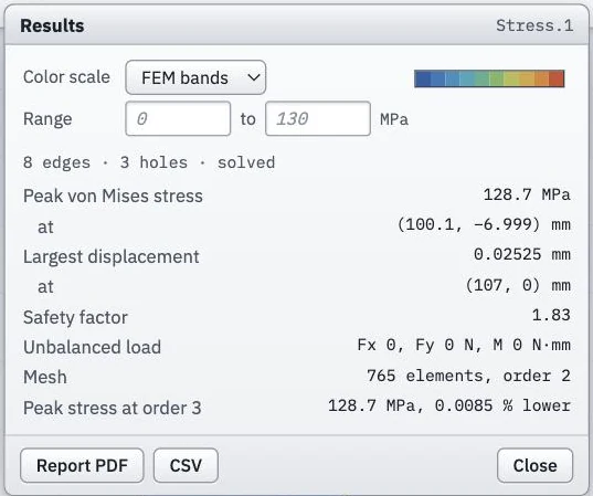
The rod’s results, with the peak stress at the next element order as a check of the mesh.
Color scale chooses the colors, FEM bands by default, the planex2d colors, Viridis or Grayscale.
Range sets the lowest and highest value of the scale. An empty box takes the value of the result, shown in gray.
Report PDF writes a two-page A4 report of the simulation: the result and its key figures on the first page, the model, the material, the mesh, the supports and loads and the measurements on the second.
CSV writes the same list as a table, with a row for each quantity.
Save as > PDF Report writes the report of a simulation chosen in a list, and solves it first if it is not up to date.
Measurements
The Measurements folder holds the values a simulation reports at places of its own choice, such as the peak stress or the hottest point, and the points and edges added to it.
Click Measurements.
Click a point in the view, or type its H and V in a new row.
Under Edges, add a row and click an edge to measure along it.
Each measurement shows its value in the view and in the tree after the next solve.
The six types
Stress analysis
The stress analysis computes a flat part in plane stress. Material sets the Young’s modulus, the Poisson’s ratio and the yield strength, from a list of materials or typed in. Solver holds the thickness, the element order, curved elements, the accuracy estimate and Balanced holding. A support is fixed, or fixed in x or in y only. A load is a force on an edge, a pressure on an edge or a hole, or a bolt load on a hole, the force of a pin in it. Show offers the von Mises stress, the displacement, the safety factor against the yield strength, the normal and shear stresses and the principal stresses.
The rod reaches 128.7 MPa at the small bore, a safety factor of 1.83 against steel S235.
Plate frequencies
Plate frequencies computes the natural frequencies and mode shapes of the part as a thin plate vibrating out of its plane. Material sets the Young’s modulus, the Poisson’s ratio and the density, and Solver the thickness and the number of modes. An edge or a hole is clamped or simply supported. Show chooses the mode, and Sand draws the mode’s nodal lines as sand gathers on a vibrating plate.
The example is an aluminum inspection cover, 2 mm thick, simply supported along its outline. Its lowest natural frequency is 172.5 Hz.
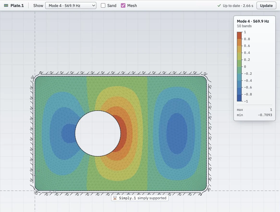
The fourth mode of the inspection cover, at 569.9 Hz.
Heat transfer
Heat transfer computes the temperatures and the heat flow. Model takes the part as the cross-section of a profile of a given length, or as a flat plate of a given thickness whose faces lose heat by convection and radiation. Regions sets the material and a heat input of each region. A boundary condition on an edge or a hole is a temperature, a heat input, convection, radiation or a contact resistance. With Transient in the Solver popup, the simulation follows the temperatures from a start temperature over a duration, and a Time slider in the results bar steps through the moments.
The example is an aluminum heat sink of 100 mm length with a copper insert that takes 20 W, cooled by convection of 8 W/m²K at 25 °C over its whole outline. The insert reaches 76.3 °C.
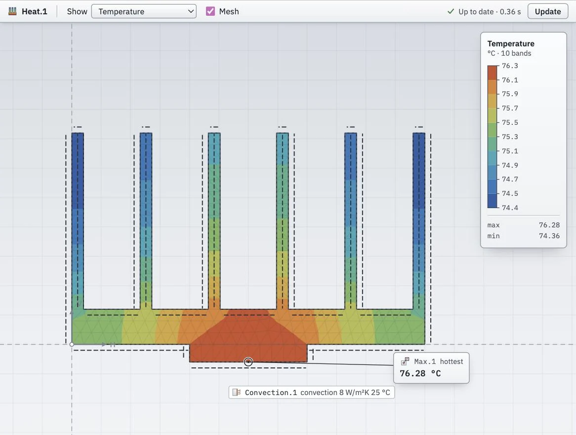
The heat sink with its copper insert, steady state.
Electrostatics
Electrostatics computes the potential, the electric field and the capacitance between conductors. Model is planar, with a length, or axisymmetric. Regions sets the dielectric of each region, or makes a region metal. A conductor is an edge, a hole or a metal region at a voltage, or a floating conductor, and an edge can carry a surface charge. Open space in the Solver popup surrounds the part with free space. The field lines start on the positively charged conductors and end on the negative ones, and lines that come from far away start on a negative conductor.
The example is a coaxial cable with a polyethylene dielectric between a conductor of 0.9 mm and a screen of 2.95 mm, at 1000 V. Its capacitance is 105.4 pF over 1000 mm, the value of the formula for a coaxial line.
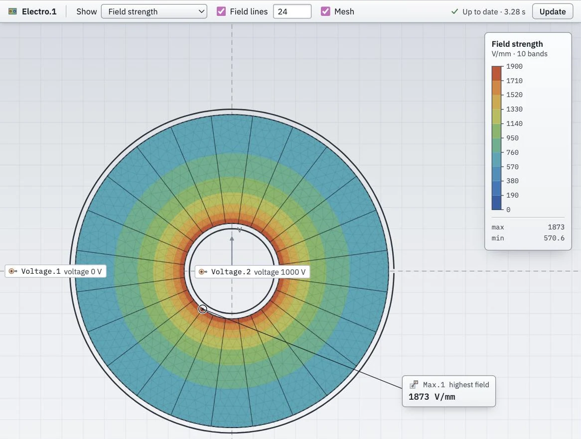
The field in the coaxial cable, strongest at the inner conductor, with its field lines.
Magnetics
Magnetics computes the magnetic field, forces and inductances, static or time-harmonic at a frequency. Regions sets the material of each region, from air and copper to electrical steel and magnet grades. Magnets gives the remanence and the direction of each magnet region. Circuits holds the currents, and Windings winds a region on a circuit with a number of turns. Flux parallel makes the flux run along an edge, such as a plane of symmetry.
The example is a Helmholtz coil, axisymmetric, two coils of 100 turns each with a current of 2 A. Between the coils the field is nearly uniform.
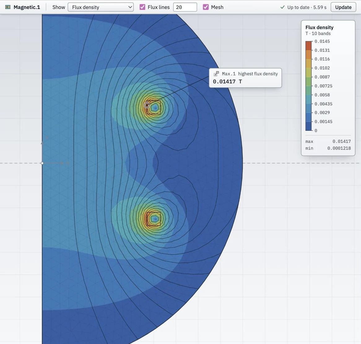
The field of the Helmholtz coil, drawn on the half plane of its axis.
Beam calculator
The beam calculator takes the result as the cross-section of a straight beam, computes its section properties, and solves the beam as an Euler-Bernoulli beam. Beam sets the length, the material and the beam’s own weight. A support is pinned or fixed at a position along the beam, and a load is a point load, a uniform load or a partial load. The results show the section above a sketch of the beam with its supports and loads, and the shear force, the bending moment and the deflection beside them. Pointing at a diagram reads its value.
The example is an IPE 200 section, 4 m long and simply supported, under 5 kN/m. The bending moment reaches 10 kNm and the deflection 4.08 mm at midspan, as 5qL⁴/(384EI) gives with the section’s second moment of area.
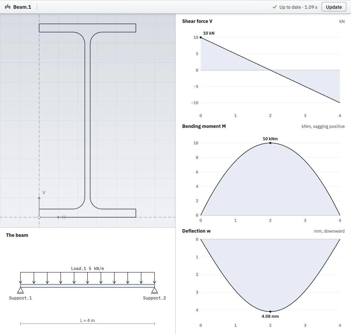
An IPE 200 section as a simply supported beam.
The project file
Save keeps each simulation’s type, input and settings in the project file, not its results. A project opens with its simulations not solved, and Solve computes them again. See Files for the project file, and the simulation tools on the site’s tools page for the same simulations on a file of their own.