Tools / PCB impedance
PCB impedance calculator
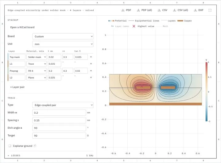
Calculate the characteristic impedance of a trace on a circuit board online and for free with a 2D field solver, for microstrip, stripline, coplanar waveguides and differential pairs. NGSolve solves the electric field of the trace's cross-section in this tab with Python, running on Pyodide/ngapp. Nothing is uploaded.
The stackup table holds the board's layers with their thickness, permittivity and loss tangent, and it can read the stackup of a KiCad board. The tool gives the impedance, the effective permittivity, the delay and the inductance and capacitance per length, for a pair the differential, common-mode, odd-mode and even-mode impedances, and the losses at a frequency. It finds the width for a target impedance and sweeps the impedance over a range of widths. A PDF report, a CSV table and a DXF file of the cross-section hold the results.
- 2D field solver
- Runs in your browser
- Built on the planex2d library
Results
Pick a board or open a KiCad board, set each layer's thickness and material, give the trace's copper layer the role Trace and the layers it refers to the role Plane, and set the trace below the table. The drawing shows the cross-section, and Solve computes the impedance. After the first solve, a changed setting solves the cross-section again. Lengths are in millimeters or mils, the frequency in GHz and the copper's conductivity in MS/m. The PDF holds the field shown and the results on an A4 sheet, the CSV file the settings and the results with the capacitance and inductance matrices, and the DXF file the cross-section. PDF (all) holds every field, and CSV (all) every field at the points of the drawing's grid.
Try a sample stackup
Each one opens in the impedance calculator above with its stackup and its trace.
-
Fig. 1Stackup
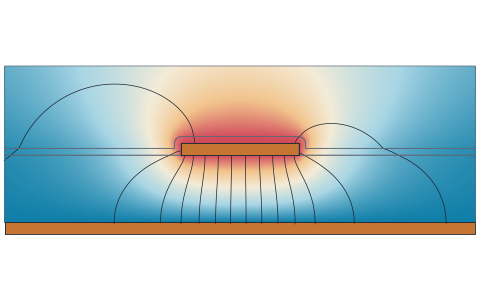
50 Ω microstrip on a 4-layer board
A microstrip on a board's top layer, over 0.2 mm of FR-4 with εr 4.3 and the ground plane on the second layer, in 35 µm copper under 20 µm of solder mask. The stackup lists only these four layers, since the field ends at the plane and the layers below it do not change the result. A trace of 0.35 mm comes out at 49.36 Ω, with an effective permittivity of 3.30 and a delay of 6.06 ps/mm, and the width for 50 Ω is 0.3416 mm. At 1 GHz it loses 4.94 dB per meter.
-
Fig. 2Stackup
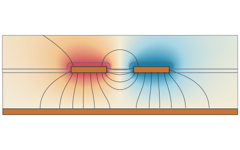
90 Ω differential pair for USB
An edge-coupled pair on the same four layers, 0.2 mm wide with a spacing of 0.15 mm, driven in the odd mode. Its differential impedance is 96.99 Ω, and the width for the 90 Ω of USB at this spacing is 0.2445 mm.
-
Fig. 3Stackup
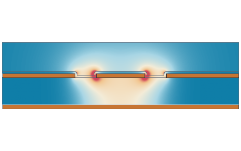
Grounded coplanar waveguide on RO4350B
A grounded coplanar waveguide on a 2-layer board of 0.254 mm RO4350B with εr 3.66, a trace of 0.45 mm with ground copper beside it at a gap of 0.2 mm, under solder mask. It comes out at 47.74 Ω, the width for 50 Ω is 0.4097 mm, and at 10 GHz it loses 12.8 dB per meter, 7.2 dB in the dielectric and 5.6 dB in the copper.
-
Fig. 4Stackup
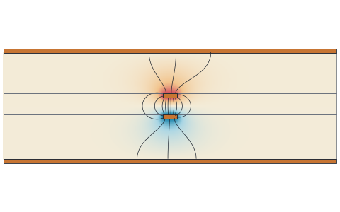
Broadside-coupled stripline
A broadside-coupled pair on the two middle layers of a 6-layer board, two traces of 0.12 mm one above the other, 0.15 mm apart, with the stackup from plane to plane. Its differential impedance is 81.02 Ω, and 100 Ω takes traces of 0.071 mm.
What the PCB impedance calculator computes
The characteristic impedance, the delay and the losses of a trace or a pair of traces on a circuit board, from the cross-section of its stackup.
A signal on a trace travels as a wave between the trace and its return path, a plane below or above it or the copper beside it. The ratio of its voltage to its current is the characteristic impedance Z0, which a trace must match to its driver and receiver for the signal to arrive without reflections. It depends on the width of the trace, its distance from the planes and the permittivity of the dielectrics around it. Closed-form formulas, such as those of Hammerstad and Jensen for the microstrip, give it for a few simple cross-sections. The tool solves the electric field of the actual cross-section with the finite element method, with the trace's thickness and etched flanks, the solder mask, several dielectrics and the copper beside the trace.
The stackup
The stackup table lists the board's layers from top to bottom, as the board house specifies them: solder mask, copper and dielectric, each with its thickness t. A dielectric layer, a core or a prepreg, has a material with its relative permittivity εr and its loss tangent tan δ. The list fills in typical values, which should be replaced by those of the laminate's data sheet at the frequency of interest. A copper layer has a role:
- Trace is the layer of the trace or the pair, and two layers have it for a broadside-coupled pair.
- Plane is a reference plane, ground or power, that runs under the whole trace.
- Unused is copper that the trace does not see, filled with the dielectric around it.
The planes nearest to the trace bound its field, and the layers beyond them do not matter. A trace with a plane on one side only is a microstrip on an outer layer, or an embedded microstrip under further dielectric. A trace between two planes is a stripline, centered or offset. The Board list fills the table with a common stackup of 2, 4 or 6 layers and 1.6 mm, + Layer pair adds a dielectric and a copper layer above the bottom one, and Open a KiCad board reads the stackup of a .kicad_pcb file.
Traces and pairs
The trace is a single trace, an edge-coupled pair side by side on one layer, or a broadside-coupled pair on two layers, one trace above the other. Its width w is the width at its base, where it sits on the dielectric, and the spacing s of an edge-coupled pair is the gap between its two traces at the base. The copper's thickness comes from the trace's layer, and a thickness of 0 gives an infinitely thin trace, as the closed-form formulas assume. With Coplanar ground on, copper at 0 V lies beside the trace or the pair on the same layer, at the gap g, and reaches out sideways without end, as a ground pour does. A microstrip with a coplanar ground is a grounded coplanar waveguide.
Solder mask and etching
A solder mask layer covers the outer copper and the dielectric between it with a coat of the layer's thickness, which follows the flanks of the trace. Since the mask puts dielectric where there was air, it lowers the impedance of an outer trace. An etched trace is narrower at its top than at its base. With an etch angle α below 90° its flanks lean in, and its top is w − 2t/tan α wide, which raises the impedance a little.
Results
For a single trace the results give its impedance Z0 and its effective permittivity εeff, the permittivity of a uniform medium in which the signal would travel as fast as on the trace. They also give the delay per length, √εeff/c, and the inductance and the capacitance per length. For a pair they give the differential impedance Zdiff between the two traces, the common-mode impedance Zcommon of both traces driven together against the planes, and the odd-mode and even-mode impedances of each trace, Zodd = Zdiff/2 and Zeven = 2·Zcommon, with the effective permittivity and the delay of both modes. For a pair whose two traces are not alike, such as a broadside pair between unequal dielectrics, these come from the impedance matrix of the two lines. The drawing colors the cross-section by the potential or the field strength, with the trace at 1 V, and a pair driven with +1 V and −1 V in the odd mode or with +1 V on both in the even mode.
Losses
With Losses on, the results add the attenuation at the frequency given, in dB per meter, or per inch when the lengths are in mils, in two parts:
- The dielectric loss comes from each dielectric's tan δ, weighted by the share of the electric field's energy in it.
- The conductor loss comes from the copper's conductivity. The current flows in a layer about a skin depth thick at the surface of the trace and of the planes, and the tool integrates its losses over every copper surface. This holds once the skin depth is small against the copper's thickness, from about 100 MHz for 35 µm copper.
The copper counts as smooth. The roughness of real copper raises the conductor loss at high frequencies and is not part of the results.
Target impedance and width sweep
With a Target, the tool searches for the trace width that gives it, Z0 for a single trace and Zdiff for a pair at the given spacing. A secant search solves the cross-section again for each width it tries and stops within 0.01 % of the target, and the results show the width with the impedance it reaches. Leave Target empty to skip the search. The width sweep solves the cross-section for a range of widths and shows the impedance over the width as a table and a chart.
KiCad boards
Open a KiCad board reads the stackup that KiCad's Board Setup saves in a .kicad_pcb file: the solder masks, the copper layers and the dielectrics with their thickness, material, εr and loss tangent, including dielectrics made of several sublayers. The first copper layer becomes the trace's layer and the second a plane, which you can change in the table. A board whose stackup was never set up in KiCad has none in its file, and the table then stays as it is. The tool reads only the stackup, not the tracks.
Units
Lengths are in millimeters or mils, as the Unit list sets them, and a change of the unit converts the table and the trace. The frequency is in GHz, the conductivity in MS/m, the delay in ps and the inductance and the capacitance per millimeter, or per inch for mils. The drawing is in millimeters, with the potential in volts and the field strength in V/mm.
How the PCB impedance calculator works
The tool is a small page around the planex2d Python library, with NGSolve for the finite element solution. It runs the same code you get with pip install "planex2d[occ]" ngsolve, compiled to WebAssembly and loaded with Pyodide/ngapp.
- Load
The page loads Python and planex2d into this tab, and NGSolve with the first solve, about 23 MB the first time. Your browser keeps them in its cache, so later visits start faster.
- Draw
planex2d draws the cross-section from the stackup and the trace, with the copper as exact polygons and the solder mask as an offset of the copper.
- Solve
NGSolve meshes the cross-section and solves its electric field with the dielectrics and in air, again whenever a setting changes after the first solve.
- Save
The results are saved as a PDF report or a CSV table, and the cross-section as a DXF file, made in the tab as well.
The finite element model
The unknown is the electric potential in the cross-section. The copper is a perfect conductor, with the traces at their voltages and the planes and the coplanar ground at 0 V. The board's layers run on sideways without end, and an open side above or below the board reaches to infinity. The tool models this with zones at the sides of the cross-section that a coordinate map stretches out to infinity along x, and zones above and below it stretched along y. The layers keep their thickness all the way out, and the result does not depend on the size of a box. For each trace, one solution with the dielectrics and one with air everywhere give the capacitance matrices C and C0 per length, the inductance matrix L = μ0ε0·C0⁻¹, and from them the impedances and the delays. The mesh is refined geometrically toward the corners of the copper, where the field is singular, 3 levels deep by default, and NGSolve solves with fourth-order elements and a sparse Cholesky factorization. Both are set in the Solver group.
How it is tested
The tests solve cross-sections whose impedance is known exactly, with infinitely thin traces as the formulas assume, and compare the tool's values with those, at its default settings. Hammerstad and Jensen's formulas are fits, which they state to hold within 0.01 % for the impedance of a microstrip in air and within 0.2 % for the effective permittivity on a substrate. The conductor loss is compared with Wheeler's incremental inductance rule, which gives the same loss from the change of the inductance when every copper surface recedes by a small step.
| Case | Reference value | The tool | Difference |
|---|---|---|---|
| Thin centered stripline, w/b 0.5, εr 4: Z0 | Cohn, 50.2162 Ω | 50.2145 Ω | 3.4 × 10⁻⁵ |
| Thin edge-coupled stripline, s/b 0.25: Zodd | Cohn, 41.7615 Ω | 41.7592 Ω | 5.5 × 10⁻⁵ |
| The same pair: Zeven | Cohn, 57.3841 Ω | 57.3824 Ω | 2.9 × 10⁻⁵ |
| Thin coplanar line in air, w 0.5, g 0.25: Z0 | conformal map, 120.484 Ω | 120.476 Ω | 7.1 × 10⁻⁵ |
| Thin microstrip in air, w/h 0.5: Z0 | Hammerstad and Jensen, 166.700 Ω | 166.672 Ω | 1.7 × 10⁻⁴ |
| Thin microstrip in air, w/h 1: Z0 | Hammerstad and Jensen, 126.424 Ω | 126.402 Ω | 1.8 × 10⁻⁴ |
| Thin microstrip in air, w/h 4: Z0 | Hammerstad and Jensen, 57.7212 Ω | 57.7149 Ω | 1.1 × 10⁻⁴ |
| Thin microstrip on εr 4.4, w/h 1: εeff | Hammerstad and Jensen, 3.16782 | 3.16889 | 3.4 × 10⁻⁴ |
| Thin microstrip on εr 4.4, w/h 4: εeff | Hammerstad and Jensen, 3.56173 | 3.56791 | 1.7 × 10⁻³ |
| Stripline in one dielectric, tan δ 0.02 at 1 GHz: dielectric loss | π f √εr tan δ / c, 3.64086 dB/m | 3.64086 dB/m | < 10⁻⁶ |
| Stripline of 0.05 mm copper at 1 GHz: resistance | Wheeler's rule, 13.4816 Ω/m | 13.5691 Ω/m | 6.5 × 10⁻³ |
| Microstrip under solder mask, etched at 70°: the width for 50 Ω | 50 Ω | 50.0002 Ω | 5 × 10⁻⁶ |
Supported files
| Format | Extensions | Notes |
|---|---|---|
| KiCad board | .kicad_pcb | The stackup of KiCad's Board Setup: solder masks, copper and dielectrics with their thickness, εr and loss tangent. See KiCad. |
.pdf | The report with the field shown, the stackup and the results on an A4 sheet. PDF (all) has every field. | |
| CSV | .csv | The settings and the results, with the capacitance, inductance and impedance matrices. CSV (all) is one table with a row for every point of the drawing's grid and every field there. |
| DXF | .dxf | The cross-section as drawn, each layer on a DXF layer of its name and the copper on the layer Copper. It opens in the electrostatics tool for cross-sections the stackup cannot describe. |
Run it in Python
The same analysis takes a few lines with planex2d and NGSolve. The example is a centered stripline, an infinitely thin strip of 0.5 mm halfway between two planes 1 mm apart, in a dielectric of εr 4. planex2d draws the space between the planes as two faces with the strip on their common edge, and NGSolve solves for the potential with the strip at 1 V and the planes and the far ends at 0 V. In a single dielectric the field energy gives the impedance directly, Z0 = √εr/(c·C) with C = ε∫|∇V|². See Meshing with netgen in the docs, and the microstrip impedance example for a microstrip and the width for 50 Ω.
$ pip install "planex2d[occ]" ngsolveimport math
import ngsolve as ngs
import planex as px
b, w, er = 1.0, 0.5, 4.0
lower = px.QuickSketch((-5, 0)).Rectangle(10, b / 2).Face()
upper = px.QuickSketch((-5, b / 2)).Rectangle(10, b / 2).Face()
strip = px.Line((-w / 2, b / 2), (w / 2, b / 2))
board = px.Glue([lower, upper, strip])
for e in board.edges:
m = e.midpoint
if strip.Distance((m.x, m.y)) < 1e-9:
e.name, e.maxh = "strip", 0.01
elif abs(m.y) < 1e-9 or abs(m.y - b) < 1e-9 or abs(abs(m.x) - 5) < 1e-9:
e.name = "ground"
mesh = ngs.Mesh(px.OCCGeometry(board).GenerateMesh(maxh=0.2))
fes = ngs.H1(mesh, order=4, dirichlet="strip|ground")
u, v = fes.TnT()
a = ngs.BilinearForm(ngs.grad(u) * ngs.grad(v) * ngs.dx).Assemble()
V = ngs.GridFunction(fes)
V.Set(1, definedon=mesh.Boundaries("strip"))
r = V.vec.CreateVector()
r.data = -a.mat * V.vec
V.vec.data += a.mat.Inverse(fes.FreeDofs(), inverse="sparsecholesky") * r
energy = ngs.Integrate(ngs.grad(V) * ngs.grad(V), mesh)
eta0 = 4e-7 * math.pi * 299792458
Z0 = eta0 / (math.sqrt(er) * energy)
def K(k):
x, y = 1.0, math.sqrt(1 - k * k)
for _ in range(8):
x, y = (x + y) / 2, math.sqrt(x * y)
return math.pi / (2 * x)
k = 1 / math.cosh(math.pi * w / (2 * b))
print("Z0", round(Z0, 3), "ohm, exact", round(eta0 / (4 * math.sqrt(er)) * K(k) / K(math.sqrt(1 - k * k)), 3))It prints an impedance of 50.176 Ω, against 50.216 Ω from Cohn's exact formula. The tool also refines the mesh toward the strip's edges, where the field is singular, and comes within 0.004 %.
Privacy
Nothing is uploaded. A KiCad file is read in this tab, only for its stackup, and is gone when you close it. Python, planex2d and its packages come from public package servers (jsDelivr and PyPI), and NGSolve from this site. See the privacy notice.
Limits
- The model is quasi-static, the field of the cross-section at rest, which holds while the cross-section is small against the wavelength. At tens of GHz the impedance and the effective permittivity change with the frequency, which the tool does not compute.
- The trace is straight and long, over planes without gaps. Vias, bends, splits in a plane and the stitching vias of a coplanar ground are not part of the model.
- The copper is smooth, and inside it the field is zero. Its roughness and the current inside it at low frequencies are left out.
- Each material has one εr and one tan δ, the values of its data sheet at the frequency of interest. The glass weave and the resin content of a real laminate vary them.
- A board that fails or a result that looks wrong? Open an issue on GitHub and attach the stackup if you can.
Questions and answers
Is my board file uploaded?
No. planex2d reads the KiCad file in this browser tab, running on Pyodide/ngapp, and NGSolve solves the field there as well. The tool reads only the stackup, and the file is gone when you close the tab. Python and its packages come from jsDelivr and PyPI, NGSolve from this site, and your file is never sent anywhere.
How wide should a 50 Ω trace be?
That depends on the stackup. A microstrip over 0.2 mm of FR-4 under solder mask is about 0.34 mm wide, and one on a two-layer board of 1.6 mm about 2.9 mm. Enter the stackup, set the target impedance to 50 Ω and press Solve. The results give the width for 50 Ω, and the width sweep shows how the impedance changes with the width.
How do I design a 90 Ω or 100 Ω differential pair?
Choose Edge-coupled pair, set the spacing s and set the target impedance to 90 or 100 Ω. The results give the width at that spacing for the differential impedance Zdiff, along with the odd-mode and even-mode impedances. A smaller spacing couples the two traces more closely and lowers Zdiff, so the same target then takes a narrower trace.
How much does the solder mask change the impedance?
On an outer trace the mask puts dielectric where there was air, and it lowers the impedance, by about 1.4 Ω for a 50 Ω microstrip under 20 µm of mask. Remove the mask layer from the table to compare. Traces on inner layers do not see it.
Why does the result differ from a closed-form calculator?
Closed-form formulas are fits for simple cross-sections, often an infinitely thin trace on a single dielectric, while the tool solves the field of the cross-section as entered. Where both apply, the tool agrees with the formulas within their stated accuracy, as the table under How it is tested shows. Differences come from the trace's thickness and etching, the solder mask, a coplanar ground or several dielectrics.
Can I use the stackup from KiCad?
Yes. Open a KiCad board reads the stackup that KiCad's Board Setup saves in a .kicad_pcb file, with the thickness, εr and loss tangent of every layer. Then pick the trace's layer and the planes in the table, and set the trace below it.
Other tools on planex2d.org
Every tool runs on the planex2d library, in your browser.
-
Electrostatics
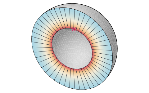
Electric fields and capacitances of cross-sections and round parts from DXF, SVG or STEP files, with dielectrics, conductors at a voltage or floating, open space and the breakdown margin.
-
Magnetics
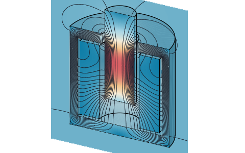
Magnetic fields, inductances and forces of cross-sections and round parts from DXF, SVG or STEP files, with B-H curves, permanent magnets, coils in circuits, eddy currents and the skin effect.
-
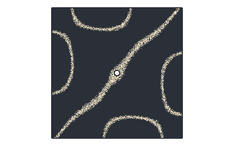
Plate frequencies
Natural frequencies and mode shapes of flat plates from DXF, SVG, STEP or KiCad files, with each edge free, clamped or simply supported, and their Chladni figures.
-
Heat transfer
Steady and transient 2D heat transfer of profiles, heat sinks and plates from DXF, SVG or STEP files, with several materials, convection, radiation and contact resistances, and the thermal resistance.
-
Playground
planex2d code in the browser, with OpenCASCADE for 3D solids and netgen and NGSolve for finite elements, shared as a link that carries the code.
The planex2d Online Tools page lists every tool, and the planex2d documentation shows the library behind them.