Tools / Heat transfer
2D heat transfer of profiles and heat sinks
Calculate the temperatures in a profile, a heat sink or a plate online and for free with the finite element method, from a DXF, SVG or STEP file. NGSolve solves the heat conduction in this tab with Python, running on Pyodide/ngapp. Nothing is uploaded. If the drawing has gaps or doubled lines, clean it in the contour checker first.
Each region of the drawing gets its own material and can generate heat, and the edges take temperatures, heat inputs, convection and radiation, with contact resistances between regions. The tool gives the temperature field, the hottest point, the heat flux and the thermal resistance in K/W, and with Transient on, how the part heats up over time. A PDF report and a CSV table hold the results.
- Steady and transient
- Runs in your browser
- Built on the planex2d library
Results
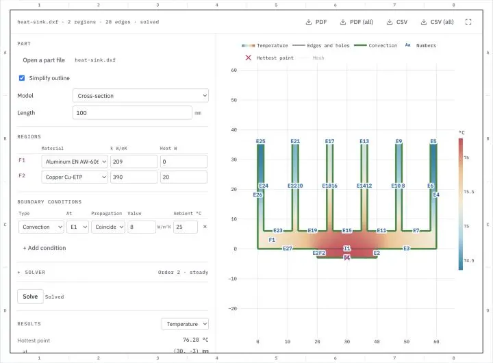
Open a part or one of the samples below, give each region its material, pick the boundary conditions by the numbers in the drawing and press Solve. After the first solve, a changed setting solves the part again. Edges and holes not in the table are insulated. Lengths are in millimeters, temperatures in °C and heat in watts. A cross-section stands for a part of the given length, and a flat plate for a plate of the given thickness, which can also be cooled over both faces. The PDF holds the field shown and the results on an A4 sheet, the CSV file the settings and the results. PDF (all) holds the temperature, the heat flux and the curve of a transient, and CSV (all) the temperature and the heat flux at the points of the drawing's grid.
Try a sample part
Each one opens in the heat transfer tool above with its materials and boundary conditions. Download them to analyze the same parts with planex2d and NGSolve in Python.
-
Fig. 1DXF
Heat sink
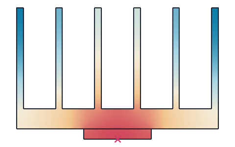
An extruded aluminum heat sink, 60 mm wide and 100 mm long with six fins 30 mm tall, and a copper heat spreader under its base that a component heats with 20 W. Natural convection with h = 8 W/m²K at 25 °C cools it all round. The hottest point, under the spreader, reaches 76.3 °C, a thermal resistance of 2.56 K/W.
-
Fig. 2DXF
Bus bar
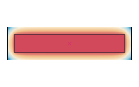
A copper bus bar of 30 × 5 mm in a 2 mm PVC sleeve, carrying about 300 A, whose Joule heating gives 10 W per meter. A contact resistance of 0.0005 K·m²/W lies between bar and sleeve, and convection with h = 10 W/m²K at 30 °C cools the sleeve. The bar reaches 43.4 °C.
-
Fig. 3DXF
Spreader plate
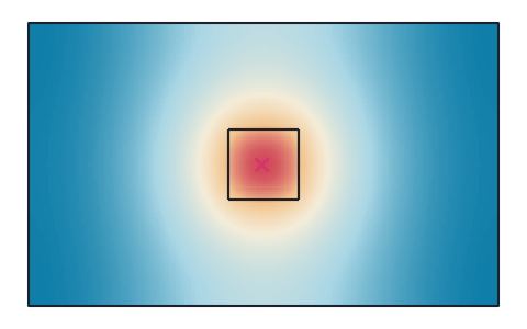
An aluminum plate of 100 × 60 × 3 mm, modeled as a flat plate, with a 15 × 15 mm component in its middle that gives off 5 W, cooled over both faces with h = 10 W/m²K at 25 °C. With Transient on, the component covers 63 % of its rise after 349 s and reaches 67.4 °C after 20 minutes, against 69.0 °C in the steady state.
What the heat transfer tool computes
The temperatures and heat flows in the cross-section of a long part or in a flat plate, from heat conduction with the boundary conditions at its edges.
Heat flows from where it is generated, in a component, a winding or a conductor, through the part to where it leaves. It leaves by convection to air or a coolant, by radiation, or into a body held at a known temperature, such as a cold plate. The temperatures along the way decide whether a component stays within its limits. Formulas give the conduction through walls, pipes and simple fins. For a real outline with several materials, the temperatures follow from a solution of the heat equation. The tool meshes the part and solves that equation with the finite element method, a steady-state or transient thermal analysis, and shows the temperature field, the hottest point and the heat leaving at every boundary.
Cross-section or flat plate
A cross-section stands for a long part, such as an extruded heat sink or a bus bar, in which the heat flows in the plane of the drawing and not along the part. The Length gives the part's length, and the results hold for that length, with the thermal resistance also per meter. A flat plate stands for a plate in which the heat spreads in its own plane, such as a spreader plate or the base of a housing. The Thickness gives the plate's thickness, and convection and radiation can act on both of its faces as well, with their values in the Part group.
Regions and materials
Every closed region of the drawing gets a number, F1, F2 and so on, and its own material with its thermal conductivity k. A loop inside another on the same layer is a hole, and a loop on a layer of its own is an insert, a region of its own material. Regions that touch exchange heat with perfect contact, unless a contact resistance is set on the edge between them. A region can also generate heat, given in watts for the whole region, such as the losses of a component or the Joule heating of a conductor.
Edge, hole and interface numbers
The outline's edges get E1, E2 and so on from the lowest left corner around the part, every hole one number for its whole boundary, H1, H2 and so on from the left, and every edge between two regions I1, I2 and so on. The boundary conditions refer to these numbers, and the drawing shows them, with each edge's length on hover. The Propagation column carries a row on along the outline, with planex2d's selection propagation.
- Minimal keeps the edge alone.
- Coincident adds the edges joined to it end to end, which on a closed outline is all of it.
- Tangent adds the edges that continue it tangentially, such as the lines on either side of a fillet.
- Curvature adds the edges that continue its curvature as well.
Boundary conditions
- A temperature holds an edge or a hole at a fixed temperature, such as a wall cooled by water.
- A heat input puts a heat flow in watts into an edge or a hole, spread evenly along it.
- Convection gives off q = h (T − T∞) to a fluid at the ambient temperature T∞, with the heat transfer coefficient h.
- Radiation gives off q = εσ (T⁴ − Ts⁴) to surroundings at Ts, with the emissivity ε. It is the radiation to open surroundings, without view factors between the part's own faces, so fins facing each other give off less than it says.
- A contact resistance R between two regions makes the temperature jump by q R across the edge between them, such as at a thermal pad or a bolted joint.
Edges and holes not in the table are insulated. Where rows meet on an edge, heat input, convection and radiation add, and a temperature overrides them.
Results
The results are the hottest and the coldest point, the heat entering the part and the heat flow through every boundary condition, which together balance. The thermal resistance is the rise of the hottest point over the lowest reference temperature, an ambient or a held temperature, divided by the heat put in, in K/W. The drawing colors the part by its temperature, or by the heat flux with the list beside Results, and marks the hottest point.
Transient
With Transient on in the Solver group, the part starts at the start temperature and heats up or cools down over the duration, in 150 time steps of the implicit Euler method. Each material then also needs its density and specific heat. The results add the curve of the hottest point over time and the time it takes to cover 63 % of its rise to the steady state, which for a small, well-conducting body is its time constant. The time slider shows the temperature field at moments across the duration, on one color scale.
Simplify outline
Drawings often carry arcs and holes as chains of short lines, which give the outline many edge numbers. With Simplify outline on, planex2d fits arcs to such chains, within a ten-thousandth of the part's size, before the part is numbered and meshed. Turn it off to analyze the outline exactly as drawn. Where the fit misses an arc, the contour checker fits arcs with a tolerance and an edge length of your choice, closes gaps and removes tiny edges, and saves the cleaned drawing for the heat transfer tool.
Units
Lengths are in millimeters, temperatures in °C, heat flows in watts, the thermal conductivity in W/mK, heat transfer coefficients in W/m²K, the density in g/cm³ and the specific heat in J/kgK. A file is read in the unit it names and converted to millimeters.
How the heat transfer tool works
The tool is a small page around the planex2d Python library, with NGSolve for the finite element solution. It runs the same code you get with pip install "planex2d[occ]" ngsolve, compiled to WebAssembly and loaded with Pyodide/ngapp.
- Load
The page loads Python and planex2d into this tab, and NGSolve with the first solve, about 23 MB the first time. Your browser keeps them in its cache, so later visits start faster.
- Read
planex2d reads the file, joins its closed contours into regions, simplifies the outline and numbers its regions, edges and holes.
- Solve
NGSolve meshes the part and solves the heat equation, again whenever a setting changes after the first solve.
- Save
The results are saved as a PDF report or a CSV table, made in the tab as well.
The finite element model
The mesh has elements of about a thirtieth of the part's size, finer along arcs, and it is curved to the exact outline. NGSolve solves the heat equation with second-order elements, set from 1 to 5 in the Solver group, and a sparse Cholesky factorization. Radiation makes the problem nonlinear, and Newton's method solves it. Across a contact resistance, each region has a temperature field of its own, coupled along the edge between them. The tests compare the tool with known answers:
- A plane wall and a pipe wall give their heat flows within 0.001 %.
- A fin, and a plate fin cooled over its faces, give the heat flow of the fin formula within 0.1 %.
- Two slabs with a contact resistance give their series resistance, and a slab heating itself its peak temperature q w² / (8 k).
- A radiating wall meets its one-dimensional energy balance, and a cooling body its time constant ρ c V / (h A) within 1 %.
Supported files
| Format | Extensions | Notes |
|---|---|---|
| DXF | .dxf | The part's lines, arcs, circles, polylines, splines and ellipses, on every layer. A closed loop on a layer of its own is an insert. See Files. |
| SVG | .svg | Paths and shapes. See SVG. |
| STEP | .step .stp | Planar parts. See STEP and BREP. |
| BREP | .brep | Planar parts, taken in meters, since BREP names no unit. |
.pdf | The report with the field shown, the settings and the results on an A4 sheet. PDF (all) has the temperature, the heat flux and the curve of a transient. | |
| CSV | .csv | The settings and the results, with the hottest point at every time step of a transient. CSV (all) is one table with a row for every point of the drawing's grid inside the part and the temperature and heat flux there. |
Run it in Python
The same analysis takes a few lines with planex2d and NGSolve. The example is the cross-section of an aluminum fin of 50 × 2 mm, its base held at 100 °C and the rest cooled with h = 10 W/m²K at 0 °C. planex2d draws the fin and names its edges, and NGSolve meshes it and solves the heat equation in millimeters, with k = 200 W/mK as 0.2 W/(mm·K) and h as 10⁻⁵ W/(mm²·K). See Meshing with netgen in the docs.
$ pip install "planex2d[occ]" ngsolveimport ngsolve as ngs
import planex as px
fin = px.QuickSketch().Rectangle(50, 2).Face()
for e in fin.edges:
e.name = "base" if e.midpoint.x == 0 else "air"
mesh = ngs.Mesh(px.OCCGeometry(fin).GenerateMesh(maxh=1))
fes = ngs.H1(mesh, order=2, dirichlet="base")
T, v = fes.TnT()
k, h = 200e-3, 10e-6
a = ngs.BilinearForm(k * ngs.grad(T) * ngs.grad(v) * ngs.dx + h * T * v * ngs.ds("air")).Assemble()
gf = ngs.GridFunction(fes)
gf.Set(100, definedon=mesh.Boundaries("base"))
r = -a.mat * gf.vec
gf.vec.data += a.mat.Inverse(fes.FreeDofs(), inverse="sparsecholesky") * r
print("heat flow", ngs.Integrate(h * gf, mesh, ngs.BND, definedon=mesh.Boundaries("air")) * 1000, "W per meter")It prints a heat flow of 97.80 W per meter of fin, against 97.80 W from the fin formula √(h P k A) θ tanh(m Lc) with the corrected length Lc = L + t/2, which counts the fin's tip.
Privacy
Nothing is uploaded. The file is read, meshed and solved in this tab and is gone when you close it. Python, planex2d and its packages come from public package servers (jsDelivr and PyPI), and NGSolve from this site. See the privacy notice.
Limits
- The tool solves heat conduction in solids with constant material values. The flow of the air or the coolant is not computed, and it enters through the heat transfer coefficient h.
- Radiation goes to open surroundings, without view factors between the part's own faces.
- A cross-section assumes no heat flow along the part, and a flat plate a temperature that does not vary through its thickness.
- The material values are typical values. Use the values of your material where they matter.
- Window frames and thermal bridges after ISO 10077-2 and ISO 10211, with their cavity rules, are not part of the tool.
- The tool analyzes one connected part. A file must be planar, and its text, dimensions and hatches are not read.
- A part that fails or a result that looks wrong? Open an issue on GitHub and attach the file if you can.
Questions and answers
Is my file uploaded?
No. planex2d reads the file in this browser tab, running on Pyodide/ngapp, and NGSolve solves the part there as well. The file is gone when you close the tab. Python and its packages come from jsDelivr and PyPI, NGSolve from this site, and your file is never sent anywhere.
How do I calculate the thermal resistance of a heat sink?
Open the heat sink's cross-section with the component, or a block under the base that stands for it, drawn as a region of its own on a layer of its own. Give that region the component's heat in watts, put convection on the outline, E1 with Coincident propagation, and enter the heat sink's length. The thermal resistance in the results is the rise of the hottest point over the ambient temperature per watt. The heat sink sample does this for a 60 mm extrusion.
Which heat transfer coefficient should I use?
It depends on the flow around the part, not on its material. Natural convection in air gives a few W/m²K, forced air from a fan some tens to a few hundred, and liquid cooling more. The tool takes h as given, so a correlation for the actual flow or a measurement gives a better result than a guess.
Is this a real finite element analysis?
Yes, of heat conduction, steady and transient. NGSolve solves the heat equation with second-order elements on a mesh of the exact outline, with several materials, generated heat, contact resistances, convection and radiation, the latter solved by Newton's method. The flow of the air or the coolant is not computed, and it enters through the heat transfer coefficient.
What does the transient show?
It shows how the part heats up or cools down from a start temperature over a given duration. The results give the hottest point over time and the time to 63 % of its rise to the steady state, which for a small, well-conducting body is its time constant ρ c V / (h A). The time slider shows the temperature field at moments across the duration.
What does Simplify outline do?
It replaces chains of short lines that follow an arc with the arc itself, within a ten-thousandth of the part's size. A hole exported as a polygon then has few edges, and the edge numbers stay few. Turn it off to analyze the outline exactly as drawn. If an arc is not found, or for more control, clean the drawing in the contour checker first. Its arc fit takes a tolerance and an edge length of your choice. It also closes gaps and removes tiny edges, and it saves the cleaned drawing as a DXF, SVG or STEP file for the heat transfer tool.
Other tools on planex2d.org
Every tool runs on the planex2d library, in your browser.
-
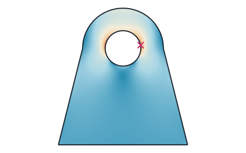
Stress analysis
Finite element stress analysis of flat parts from DXF, SVG or STEP files, with supports and loads by edge and hole number, the von Mises and principal stresses, the deformed shape and a safety factor.
-
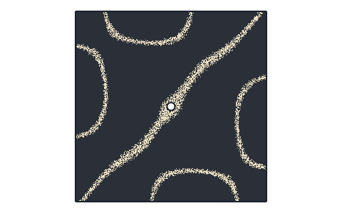
Plate frequencies
Natural frequencies and mode shapes of flat plates from DXF, SVG, STEP or KiCad files, with each edge free, clamped or simply supported, and their Chladni figures.
-
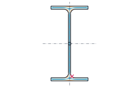
Section properties
Area, centroid, second moments and section moduli of any drawn or standard section, the mass of a sheet part, and the torsion constant and shear center from a finite element solve.
-
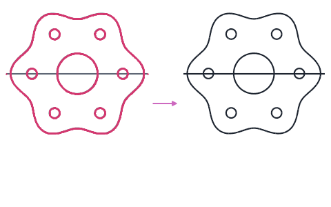
Contour checker
Open contours, gaps, doubled lines and tiny edges found in DXF, SVG and STEP drawings and repaired, with arcs fitted to tessellated outlines.
-
Playground
planex2d code in the browser, with OpenCASCADE for 3D solids and netgen and NGSolve for finite elements, shared as a link that carries the code.
The planex2d Online Tools page lists every tool, and the planex2d documentation shows the library behind them.