Tools / Magnetics
2D magnetics
Calculate the magnetic field, the forces and the inductance of a cross-section or a rotationally symmetric part online and for free with the finite element method, from a DXF, SVG or STEP file. NGSolve solves the magnetic field in this tab with Python, running on Pyodide/ngapp. Nothing is uploaded. If the drawing has gaps or doubled lines, clean it in the contour checker first.
Each region of the drawing gets its material, air, a conductor, iron on its B-H curve or a permanent magnet, and the coils carry their currents in circuits. The tool gives the flux density and the field intensity, the flux linkage and the inductance of every circuit, the force and the torque on a moving part and the stored energy. At a frequency it adds the eddy currents, the skin effect and the losses. A PDF report and a CSV table hold the results.
- Static and time-harmonic
- Runs in your browser
- Built on the planex2d library
Results
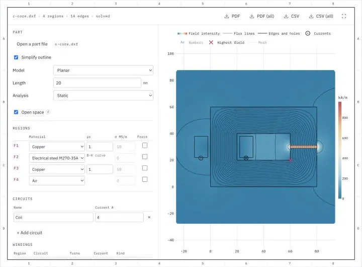
Open a part or one of the samples below, give each region its material, add a circuit with its current, give the coil regions their circuit, turns and direction in the Windings table by the numbers in the drawing, and press Solve. After the first solve, a changed setting solves the part again. Regions and edges added under Measurements show their values in the results. Edges not in the Flux parallel table are open to the flux, which crosses them at right angles, as on a plane of symmetry, and holes are filled with air. Lengths are in millimeters, currents in amperes, as amplitudes in time-harmonic mode, conductivities in MS/m and the remanence in tesla. The PDF holds the field shown and the results on an A4 sheet, the CSV file the settings and the results. PDF (all) holds every field, and CSV (all) every field at the points of the drawing's grid.
Try a sample part
Each one opens in the magnetics tool above with its materials, circuits and windings. Download them to analyze the same parts with planex2d and NGSolve in Python.
-
Fig. 1DXF
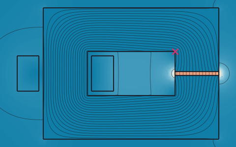
C core with an air gap
A C core of M270-35A electrical steel, 80 × 60 mm with limbs of 20 mm and a stack of 20 mm, with an air gap of 2 mm in one limb and a coil of 400 turns at 4 A on the opposite limb, in open space. The field intensity in the gap comes out at 783 kA/m, a flux density of 0.98 T, against N·I/g = 800 kA/m for a core of infinite permeability, and the coil's inductance is 57.7 mH.
-
Fig. 2DXF
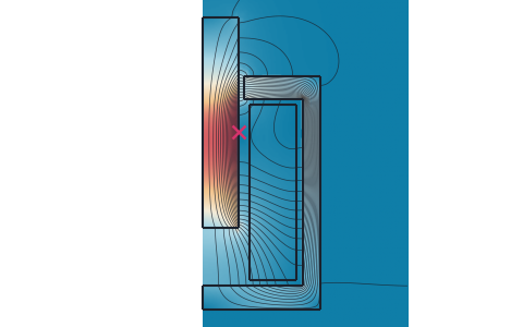
Solenoid actuator
A solenoid actuator, a steel frame of 40 mm diameter with a coil of 600 turns at 2 A and a steel plunger that ends 10 mm above the frame's bottom, solved as an axisymmetric part in open space. The coil pulls the plunger in with 2.98 N, and its inductance in this position is 18.9 mH.
-
Fig. 3DXF
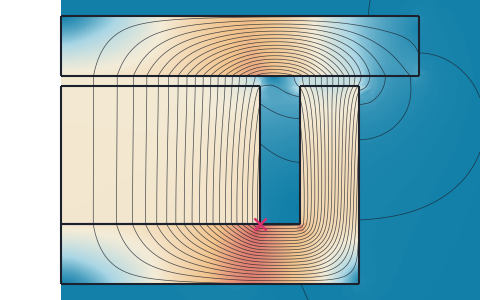
Pot magnet
A pot magnet, an N42 disc of 20 mm diameter and 7 mm height in a steel cup of 30 mm, holding a steel plate across a gap of 0.5 mm, axisymmetric in open space. The plate is held with 197 N, with a mean flux density of 0.99 T in the plate and 1.26 T in the cup.
-
Fig. 4DXF
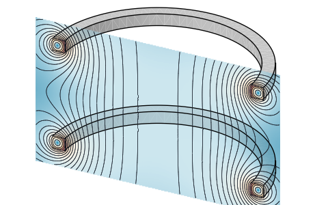
Helmholtz coil
A Helmholtz coil, two coils of 100 turns at 2 A on a radius of 50 mm, one radius apart, axisymmetric in open space. The field at the center is 3.596 mT, within 0.03 % of 0.7155·μ0·N·I/R for thin coils, and a quarter radius from the center along the axis it is 0.46 % lower. Between the coils the flux lines run almost parallel.
-
Fig. 5DXF
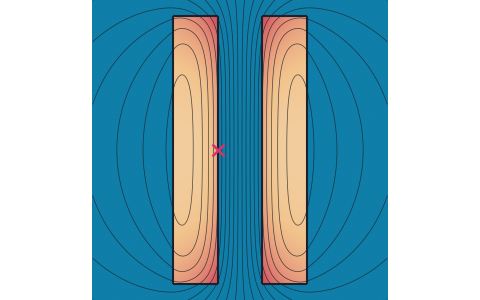
Bus bars at 50 Hz
Two copper bus bars of 60 × 10 mm, 10 mm apart, carrying a current of 1000 A amplitude at 50 Hz there and back, solved as solid conductors in open space. The current crowds toward the facing sides, and the resistance of 1 m of the pair is 60.9 µΩ, 6 % above its DC resistance of 57.5 µΩ, with losses of 30.5 W and an inductance of 235 nH.
What the magnetics tool computes
The magnetic field of coils and permanent magnets in iron, air and conductors, in the cross-section of a long part or in a rotationally symmetric part, with the inductances, forces and losses that follow from it.
Currents in coils and the magnetization of permanent magnets set up a magnetic field, which iron guides along its paths and air gaps resist. The flux density decides whether the iron saturates, the field in an air gap the force on an armature, and the flux through a coil its inductance. Formulas give these for a few shapes, such as a long solenoid or a magnetic circuit with a narrow gap, as long as the iron is far from saturation. For a real cross-section with its leakage flux, its fringing at the gaps and its saturation, they follow from a solution of the magnetic field equation. The tool meshes the part and solves that equation with the finite element method, and shows the flux density, the field intensity and the flux lines.
Planar or axisymmetric
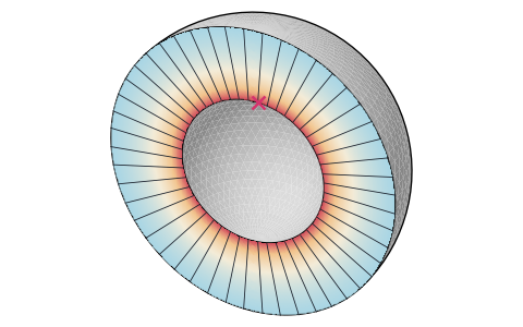
A planar model stands for a long part, such as a laminated core, a motor section, a cable or a bus bar, in which the field lies in the plane of the drawing and the currents run across it. The Length gives the part's length, the depth of a laminated stack for example, and the inductances and forces hold for that length and also per meter. An axisymmetric model stands for a part that is round about an axis, such as a solenoid, a pot magnet or a coil on a round core. The drawing is then the half-section right of its y axis, which is the axis of rotation, the currents run around the axis, and the results hold for the whole part. With 3D on, the drawing shows the part revolved through half a turn, seen at an angle, with the field and the flux lines on its cut face on both sides of the axis.
Static or time-harmonic
The static analysis solves for direct currents and permanent magnets, with iron on its B-H curve. The time-harmonic analysis solves for currents that alternate at one frequency, with the eddy currents they induce in conductors. See the section on the time-harmonic analysis below for what changes there.
Regions and materials
Every closed region of the drawing gets a number, F1, F2 and so on, and a material from the list. A loop inside another on the same layer is a hole, and a loop on a layer of its own is an insert, a region of its own material. Regions that touch must lie on layers of their own, and holes are filled with air.
- Air and the non-magnetic conductors, copper, aluminum, brass and stainless steel, have a relative permeability μr of 1. Their electrical conductivity σ counts in the time-harmonic analysis.
- Electrical steel, structural steel, cast iron and soft ferrite follow typical B-H curves, so their permeability falls as they saturate. B-H curve from a file takes the curve of a data sheet as a CSV file with the columns B in tesla and H in A/m. Linear takes a constant μr.
- The permanent magnets have their typical remanence Br and recoil permeability μr, which the Magnets table shows and lets you change. Each magnet is magnetized along an angle from the x axis, or radially out of or into the drawing's origin, as in the rotor of a motor.
Circuits and windings
A circuit carries a current, and its windings are the regions that the current flows through. Each winding has its circuit, its number of turns and the direction of its current, out of the drawing or into it, and a coil's current density is the turns times the current over the region's area. In a planar model a coil appears twice, as the side where its turns go into the drawing and the side where they come back, and both belong to the same circuit, so that its flux linkage and inductance come out right. A circuit whose currents do not add up to zero in a planar drawing has its return path outside, and its inductance is left out. In an axisymmetric model a coil is a single region, since its turns run around the axis. With several circuits the results also give the mutual inductances.
Edge, hole and interface numbers
The outline's edges get E1, E2 and so on from the lowest left corner around the part, every hole one number for its whole boundary, H1, H2 and so on from the left, and every edge between two regions I1, I2 and so on. The Flux parallel table refers to these numbers, and the drawing shows them, with each edge's length on hover. The Propagation column carries a row on along the outline, with planex2d's selection propagation.
- Minimal keeps the edge alone.
- Coincident adds the edges joined to it end to end, which on a closed outline is all of it.
- Tangent adds the edges that continue it tangentially, such as the lines on either side of a fillet.
- Curvature adds the edges that continue its curvature as well.
Boundaries and open space
With Open space on, the part sits in air that reaches to infinity, as a core or a coil does on a test bench. The tool adds an air region around the drawing, and around that a thin layer whose coordinates a map stretches out to infinity, where the field vanishes. The result is then that of all the space outside and does not depend on the size of a box. Without it, the drawing's outline bounds the field. Edges in the Flux parallel table hold the vector potential at zero, so the flux runs along them and none crosses, as at the edge of a magnetic shield. The other edges are open to the flux, which crosses them at right angles, as on a plane of symmetry between two poles. In an axisymmetric model the axis is always flux parallel.
Forces and torque
The Force column marks the regions of a moving part, such as the armature of an electromagnet, the plunger of a solenoid or a plate held by a magnet. The tool integrates the Maxwell stress tensor over the air around the part, weighted by a function that falls from 1 on the part to 0 away from it, and gets the force on the whole part from it. In a planar model the result is the force in x and y and the torque about the drawing's origin, and in an axisymmetric model the force along the axis. The moving part needs air around it, a region of air or the open space, and must not touch iron that does not move with it.
Measurements
The Measurements group, folded below the tables, adds values for the regions and edges you choose to the results.
- A region gives its mean flux density and mean field intensity and its highest flux density, for iron with the relative permeability there, and in the time-harmonic analysis its losses and skin depth. A region drawn in an air gap thus gives the field in that gap.
- An edge, a hole or an interface, carried on with the Propagation column, gives its length, the flux across it, the mean normal flux density and the magnetic voltage ∫H·dl along it. The flux across is per the Length in a planar model and through the surface of revolution in an axisymmetric one, and ∫H·dl around a closed loop is the current inside it.
Results
For each circuit the results give its flux linkage and its inductance. With iron on a B-H curve the inductance is the flux linkage over the current at that current, so it falls as the iron saturates. They also give the force and the torque on the moving part, the energy stored in the field and the highest flux density with its place. The PDF and the CSV file also list every region with its mean and highest flux density. The drawing colors the field by the flux density, its components, the field intensity, the flux function, the relative permeability, the current density or the energy density with the list beside Results. The flux lines are lines of the flux function, as many as the number beside Results, with the same flux between each pair of them, so they crowd where the field is strong.
At a sharp inner corner of iron the flux density of a magnetic solution grows without limit, so the highest flux density there depends on the mesh. The accuracy estimate in the Solver group shows this as a large change, and the mean values of the regions are not affected.
The time-harmonic analysis
In the time-harmonic analysis all currents alternate at the frequency given, and the currents are their amplitudes. Every conductor with a conductivity carries eddy currents, and a winding is either stranded or solid.
- A stranded winding is a coil of thin wire, whose current spreads evenly over its area. Its own wire resistance depends on the wire and is not part of the results.
- A solid winding is one conductor, such as a bus bar or a cable core, whose current the skin and proximity effects push to its surface and away from its neighbors. Its turns are 1.
- A conductor in no circuit carries eddy currents only, with no net current in a planar model, and in an axisymmetric model as a ring around the axis.
The results give each circuit's resistance and inductance at that frequency, the losses in every conductor and in total, and the skin depth of its material. The drawing adds the loss density, and the fields are their amplitudes. Iron is linear in this analysis, with the initial permeability of its curve, electrical steel counts as laminated with no eddy currents across the stack, and magnets count with their recoil permeability only, since a constant magnetization adds nothing at the frequency.
Simplify outline
Drawings often carry arcs and holes as chains of short lines, which give the outline many edge numbers. With Simplify outline on, planex2d fits arcs to such chains, within a ten-thousandth of the part's size, before the part is numbered and meshed. Turn it off to analyze the outline exactly as drawn. Where the fit misses an arc, the contour checker fits arcs with a tolerance and an edge length of your choice, closes gaps and removes tiny edges, and saves the cleaned drawing for the magnetics tool.
Units
Lengths are in millimeters, currents in amperes, frequencies in hertz, conductivities in MS/m, the flux density and the remanence in tesla, the field intensity in A/m and kA/m, the current density in A/mm², the energy density in J/m³ and the loss density in W/cm³. The flux function is in mWb/m in a planar model and in mWb, the flux through the circle about the axis, in an axisymmetric model. A file is read in the unit it names and converted to millimeters.
How the magnetics tool works
The tool is a small page around the planex2d Python library, with NGSolve for the finite element solution. It runs the same code you get with pip install "planex2d[occ]" ngsolve, compiled to WebAssembly and loaded with Pyodide/ngapp.
- Load
The page loads Python and planex2d into this tab, and NGSolve with the first solve, about 23 MB the first time. Your browser keeps them in its cache, so later visits start faster.
- Read
planex2d reads the file, joins its closed contours into regions, simplifies the outline and numbers its regions, edges and holes.
- Solve
NGSolve meshes the part and solves the magnetic field equation, again whenever a setting changes after the first solve.
- Save
The results are saved as a PDF report or a CSV table, made in the tab as well.
The finite element model
The unknown is the magnetic vector potential, the component along the part in a planar model and around the axis in an axisymmetric one, whose lines of constant value are the flux lines. The mesh has elements of about a thirtieth of the part's size, finer along arcs and short edges and within a skin depth of a conductor's surface, and it is curved to the exact outline. The hp refinement in the Solver group refines the mesh geometrically toward every vertex and edge of the part, as many levels deep as given, since the field changes fastest there, and it integrates the refined elements with a higher order. It is off by default, and 3 levels sharpen the field at sharp corners. NGSolve solves with second-order elements, set from 1 to 5 in the Solver group, and a sparse Cholesky factorization. With iron on a B-H curve the tool minimizes the field's energy with Newton's method, and it finds the inductances with the permeability of that solution held fixed. In the time-harmonic analysis it solves once for the given currents and once for each solid conductor, and combines these solutions so that each conductor carries its current.
How it is tested
The tests solve parts whose field, inductance or force is known exactly and compare the tool's values with those, with second-order elements, and third-order elements for the field outside the magnetized sphere. The saturated steel sleeve is a coaxial cable with a sleeve of structural steel in its insulation, where the field intensity is I/(2πr) in any material, so the flux density follows from the B-H curve alone. A further test compares the force on an electromagnet's armature with the stress tensor on a contour around it, which agrees within 1.2 %.
| Case | Exact value | The tool | Difference |
|---|---|---|---|
| Coaxial cable, core 2 mm, tube 7 to 8 mm: inductance | μ0/2π (¼ + ln(b/a) + tube) = 310.05889 nH/m | 310.05801 nH/m | 2.9 × 10⁻⁶ |
| The same cable at 10 A: mean field intensity in the insulation | I/(π(a + b)) = 707.355 A/m | 707.339 A/m | 2.3 × 10⁻⁵ |
| The same cable: ∮H·dl measured around the core | I = 10 A | 9.96554 A | 3.4 × 10⁻³ |
| A ferrite sleeve of μr 50 in the insulation: inductance | closed form, 5316.2545 nH/m | 5315.8831 nH/m | 7.0 × 10⁻⁵ |
| A steel sleeve at 50 A, saturated: flux density at its inner surface | B-H curve at H = I/(2πr), 1.6202 T | 1.6282 T | 4.9 × 10⁻³ |
| The steel sleeve at 50 A: inductance Ψ/I | field of H = I/(2πr), 31272.36 nH/m | 31269.60 nH/m | 8.8 × 10⁻⁵ |
| Two-wire line in open space, d/a = 10: inductance | μ0/π (¼ + ln(d/a)) = 1021.034 nH/m | 1020.940 nH/m | 9.2 × 10⁻⁵ |
| The same line at 100 A: force between the wires | μ0I²/(2πd) = 0.200000 N/m | 0.199969 N/m | 1.6 × 10⁻⁴ |
| Thick solenoid in open space, axisymmetric: field at its center | closed form, 7.87634 mT | 7.87610 mT | 3.1 × 10⁻⁵ |
| Helmholtz coil, coils of 6 × 6 mm: field at its center | closed form, 3.59585 mT | 3.59580 mT | 1.5 × 10⁻⁵ |
| Magnetized sphere, Br 1.2 T, μr 1.05: field inside | 2Br/(μr + 2) = 0.786885 T | 0.786890 T | 6.0 × 10⁻⁶ |
| The same sphere: field on the axis at 1.5 radii | dipole, 0.23315 T | 0.23320 T | 2.1 × 10⁻⁴ |
| Round copper wire at 40 kHz, radius 3 skin depths: AC resistance | Bessel functions J0/J1, 9.77942 mΩ/m | 9.78007 mΩ/m | 6.6 × 10⁻⁵ |
| The same wire: inductance | Bessel functions J0/J1, 292.3300 nH/m | 292.3427 nH/m | 4.3 × 10⁻⁵ |
Supported files
| Format | Extensions | Notes |
|---|---|---|
| DXF | .dxf | The part's lines, arcs, circles, polylines, splines and ellipses, on every layer. A closed loop on a layer of its own is an insert. See Files. |
| SVG | .svg | Paths and shapes. See SVG. |
| STEP | .step .stp | Planar parts. See STEP and BREP. |
| BREP | .brep | Planar parts, taken in meters, since BREP names no unit. |
| CSV | .csv .txt | A B-H curve for a region, two columns B in T and H in A/m, from zero up. |
.pdf | The report with the field shown, the settings and the results on an A4 sheet. PDF (all) has every field. | |
| CSV | .csv | The settings and the results, with the inductance matrix. CSV (all) is one table with a row for every point of the drawing's grid in the field and every field there. |
Run it in Python
The same analysis takes a few lines with planex2d and NGSolve. The example is a coaxial cable with a copper core of 2 mm diameter and a copper tube from 7 to 8 mm, with 1 A going out through the core and back through the tube. planex2d draws the section as three glued regions and names the outer edge, and NGSolve meshes it and solves for the vector potential with A = 0 outside. The integral of A times the current density then gives the inductance per meter, L = ∫A·J for 1 A. See Meshing with netgen in the docs, and the surface magnet motor example for a magnetic field in a motor's lamination.
$ pip install "planex2d[occ]" ngsolveimport math
import ngsolve as ngs
import planex as px
core = px.Circle((0, 0), 1).Face()
gap = px.QuickSketch().Circle(3.5).Circle(1).Face()
tube = px.QuickSketch().Circle(4).Circle(3.5).Face()
core.name, gap.name, tube.name = "core", "gap", "tube"
cable = px.Glue([core, gap, tube])
for e in cable.edges:
if abs(e.mass - 8 * math.pi) < 1e-6:
e.name = "outside"
mesh = ngs.Mesh(px.OCCGeometry(cable).GenerateMesh(maxh=0.2))
mesh.Curve(2)
mu0 = 4e-7 * math.pi
J = mesh.MaterialCF({"core": 1 / (math.pi * 1e-6), "tube": -1 / (math.pi * (4**2 - 3.5**2) * 1e-6)}, default=0)
fes = ngs.H1(mesh, order=2, dirichlet="outside")
u, v = fes.TnT()
a = ngs.BilinearForm(ngs.grad(u) * ngs.grad(v) * ngs.dx).Assemble()
f = ngs.LinearForm(mu0 * 1e-6 * J * v * ngs.dx).Assemble()
A = ngs.GridFunction(fes)
A.vec.data = a.mat.Inverse(fes.FreeDofs(), inverse="sparsecholesky") * f.vec
L = ngs.Integrate(A * J * 1e-6, mesh)
b, c = 3.5, 4
exact = mu0 / (2 * math.pi) * (0.25 + math.log(b) + c**4 * math.log(c / b) / (c**2 - b**2) ** 2
- (3 * c**2 - b**2) / (4 * (c**2 - b**2)))
print("L", round(L * 1e9, 3), "nH/m, exact", round(exact * 1e9, 3))It prints an inductance of 310.058 nH per meter, against 310.059 nH from the closed form.
Privacy
Nothing is uploaded. The file is read, meshed and solved in this tab and is gone when you close it. Python, planex2d and its packages come from public package servers (jsDelivr and PyPI), and NGSolve from this site. See the privacy notice.
Limits
- A planar model assumes a field that does not change along the part, with no end effects of a finite stack, and an axisymmetric model a part and a field that are round about the y axis.
- The circuits are driven by their currents. Voltage sources, moving parts and transients are not computed, and the part is solved in the position drawn.
- Magnets follow their recoil line and do not demagnetize. Hysteresis and the core losses of laminated steel are not computed, and iron is linear in the time-harmonic analysis.
- The B-H curves of the list are typical values. Load the curve of the data sheet as a CSV file where the exact steel matters.
- The flux density at a sharp inner corner of iron depends on the mesh, and a file must be planar, and its text, dimensions and hatches are not read.
- A part that fails or a result that looks wrong? Open an issue on GitHub and attach the file if you can.
Questions and answers
Is my file uploaded?
No. planex2d reads the file in this browser tab, running on Pyodide/ngapp, and NGSolve solves the field there as well. The file is gone when you close the tab. Python and its packages come from jsDelivr and PyPI, NGSolve from this site, and your file is never sent anywhere.
How do I calculate the inductance of a coil?
Draw the coil's cross-section, in a planar model both of its sides, the one going into the drawing and the one coming back, and in an axisymmetric model one region beside the axis. Add a circuit with the current and give each coil region its circuit, its turns and its direction in the Windings table. The results give the flux linkage and the inductance, for an iron core on its B-H curve the inductance at that current.
How do I get the force of an electromagnet or a magnet?
Tick Force for the regions of the moving part, such as an armature or a plunger, and make sure air surrounds it, as a region of air or the open space. The tool integrates the Maxwell stress tensor in the air around the part and gives the force on it, and in a planar model also the torque about the drawing's origin.
What does the B-H curve file need?
A CSV file with two columns, B in tesla and H in A/m, one point per line from zero up, as a data sheet lists them. A header row is allowed, columns named B and H are found by their names, and a file separated by semicolons may use decimal commas. Beyond its last point the curve continues with the slope of air.
What does the time-harmonic mode compute?
The field at one frequency, with all currents sinusoidal. Conductors carry eddy currents, solid conductors in a circuit spread their current by the skin and proximity effects, and the results give each circuit's resistance and inductance at that frequency and the losses in every conductor. Iron is linear there, with the initial permeability of its curve, and laminated electrical steel carries no eddy currents.
Is this a real finite element analysis?
Yes. NGSolve solves the equation for the magnetic vector potential with second-order elements on a mesh of the exact outline, with B-H curves, permanent magnets, coils and eddy currents, planar or axisymmetric. The tests compare it with the exact fields and inductances of coaxial cables, a two-wire line, a thick solenoid, a Helmholtz coil, a magnetized sphere and a round wire at 40 kHz.
Other tools on planex2d.org
Every tool runs on the planex2d library, in your browser.
-
Electrostatics
Electric fields and capacitances of cross-sections and round parts from DXF, SVG or STEP files, with dielectrics, conductors at a voltage or floating, open space and the breakdown margin.
-
PCB impedance
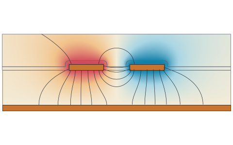
Characteristic and differential impedance of microstrip, stripline and coplanar traces from the board stackup or a KiCad board, with losses and the width for a target impedance.
-
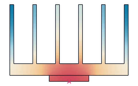
Heat transfer
Steady and transient 2D heat transfer of profiles, heat sinks and plates from DXF, SVG or STEP files, with several materials, convection, radiation and contact resistances, and the thermal resistance.
-
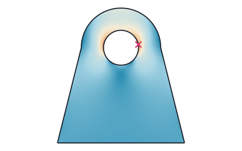
Stress analysis
Finite element stress analysis of flat parts from DXF, SVG or STEP files, with supports and loads by edge and hole number, the von Mises and principal stresses, the deformed shape and a safety factor.
-
Playground
planex2d code in the browser, with OpenCASCADE for 3D solids and netgen and NGSolve for finite elements, shared as a link that carries the code.
The planex2d Online Tools page lists every tool, and the planex2d documentation shows the library behind them.