Tools / Plate frequencies
Natural frequencies of plates
Calculate the natural frequencies and mode shapes of a flat plate online and for free with the finite element method, from a DXF, SVG, STEP or KiCad file. NGSolve solves the plate's vibration in this tab with Python, running on Pyodide/ngapp. Nothing is uploaded. If the drawing has gaps or doubled lines, clean it in the contour checker first.
Each edge and hole of the plate is free, clamped or simply supported, so the tool covers a Chladni plate as well as a circuit board on its mounting screws or a cover bolted in place. Each mode shows its deflection and its nodal lines, the Chladni figure where sand would gather, and a play button sounds its frequency. A PDF report shows the modes, a CSV table lists the frequencies, and a DXF or SVG file holds the nodal lines.
- Plate modal analysis
- Runs in your browser
- Built on the planex2d library
Modes
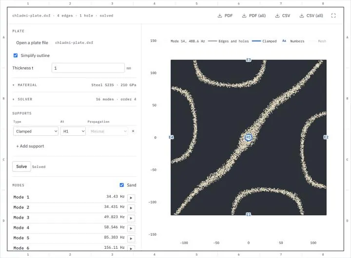
Open a plate or one of the samples below, pick the supports by the numbers in the drawing and press Solve. After the first solve, a changed setting solves the plate again. Edges and holes not in the supports table are free. Lengths are in millimeters and frequencies in hertz. A click on a mode shows it, its play button sounds it, and Sand draws its nodal lines as sand on a dark plate. The PDF holds the mode shown and the frequencies on an A4 sheet, the CSV file the settings and the frequencies. PDF (all) holds one such sheet for every mode, in the look the Sand switch sets, and CSV (all) every mode's deflection at the points of the drawing's grid.
Try a sample plate
Each one opens in the plate tool above with its material and supports. Download them to analyze the same plates with planex2d and NGSolve in Python.
-
Fig. 1DXF
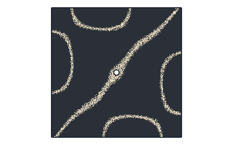
Chladni plate
A steel plate of 240 × 240 × 1 mm, clamped at a 10 mm hole in its middle, the way a Chladni plate sits on the post of its stand. Its two lowest modes share 34.4 Hz, and the next lie at 49.8 and 58.5 Hz. The picture shows mode 14, at 488.6 Hz with Modes set to 14, in the Sand look.
-
Fig. 2KiCad
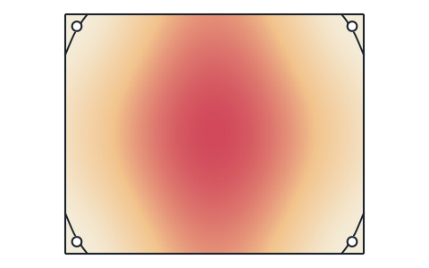
Circuit board
A board of 100 × 80 mm in 1.6 mm FR-4 from a KiCad file, screwed down at its four mounting holes. Its first mode, at 490 Hz, bows the middle of the board. The tool reads the outline and the holes and leaves out the ten vias.
-
Fig. 3DXF
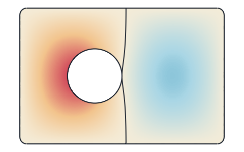
Inspection cover
An aluminum cover of 300 × 200 × 2 mm with an 80 mm opening, simply supported all round by one support row with Coincident propagation. Its first mode lies at 172.5 Hz, and the second, in the picture, at 334.5 Hz, with one nodal line across the cover.
What the plate tool computes
The natural frequencies and mode shapes of a flat plate vibrating out of its plane, with its edges free, clamped or simply supported.
A plate vibrates freely at its natural frequencies, each with a shape of its own, the mode shape. Near one of them, a small periodic force, such as from a motor, a fan or a vehicle, makes the plate vibrate strongly in resonance, so a design keeps the natural frequencies clear of the excitation frequencies. Formula collections give the frequencies of rectangular and circular plates with standard supports. For any other outline, with holes and supports on parts of its edges, they follow from the eigenvalue problem of the plate's equations of motion. The tool meshes the plate, solves that problem with the finite element method, which is a modal analysis, and shows each mode with its frequency and its nodal lines.
Chladni figures
Ernst Chladni strewed sand on metal plates and bowed their edges. At a natural frequency, the plate vibrates in one of its modes, and the sand gathers on the nodal lines, where the plate stands still. The tool draws each mode's deflection in color, red on one side and blue on the other, with the nodal lines dark where the deflection changes its sign. With Sand on, it shows the plate dark and the sand along the nodal lines instead, where the deflection is small. A mode that moves to one side everywhere has no nodal line, such as the third mode of the Chladni plate sample, which is clamped at its middle.
The plate model
The plate is a Reissner-Mindlin plate, whose deflection w and rotations are unknowns of their own, coupled by the shear. For a thin plate, the model gives the frequencies of Kirchhoff's classic thin plate theory, and for a thicker one, it includes the shear deformation and the rotary inertia, which lower the higher frequencies. The material enters through Young's modulus E, Poisson's ratio ν and the density ρ, and the thickness t through the bending stiffness D = E t³ / (12 (1 − ν²)). For a thin plate, every frequency grows in proportion to the thickness.
Edge and hole numbers
Every edge of the outline gets a number, from E1 at the lowest left corner around the plate, and every hole one number for its whole boundary, H1, H2 and so on from the left. The supports refer to these numbers, and the drawing shows them, with each edge's length and each hole's size on hover. The Propagation column carries a support on along the outline, with planex2d's selection propagation.
- Minimal keeps the edge alone.
- Coincident adds the edges joined to it end to end, which on a closed outline is all of it.
- Tangent adds the edges that continue it tangentially, such as the lines on either side of a fillet.
- Curvature adds the edges that continue its curvature as well.
Supports
A clamped edge or hole can neither move nor turn. A simply supported one cannot move out of the plane but can turn about the edge, like a plate resting on a knife edge. Edges and holes not in the table are free. A clamped hole stands for a screw or a post that holds the plate. The supports are edges and holes, not single points, so a standoff is a small hole drawn at its place and clamped. A free plate has three rigid-body modes at zero frequency, in which it moves up and down or tilts as a whole without bending, and the tool leaves them out.
Results
The results are the frequencies of the lowest modes, eight by default, the plate's mass and the mesh. A click on a mode shows it in the drawing, and its play button sounds its frequency for a moment, for frequencies from 20 Hz to 20 kHz. The deflection of each mode is scaled so that its largest value is 1, since a mode gives the shape of the vibration and not its size. The nodal lines of the mode shown can be saved as a DXF or SVG file, with the plate's outline on a layer of its own, for example to engrave the figure. The PDF report draws the modes in the look the Sand switch sets.
KiCad boards
A KiCad board (.kicad_pcb, KiCad 9 and later) gives its outline on Edge.Cuts and the holes through the board. Holes under 2 mm across, such as vias and the holes of component pins, are left out, since they change the frequencies little and would need a very fine mesh. Components add mass and some stiffness, which usually lowers the frequencies of a populated board below those of the bare board the tool computes.
Simplify outline
Drawings often carry arcs and holes as chains of short lines, which give the outline many edge numbers. With Simplify outline on, planex2d fits arcs to such chains, within a ten-thousandth of the plate's size, before the plate is numbered and meshed. Turn it off to analyze the outline exactly as drawn. Where the fit misses an arc, the contour checker fits arcs with a tolerance and an edge length of your choice, closes gaps and removes tiny edges, and saves the cleaned drawing for the plate tool.
Units
Lengths are in millimeters, Young's modulus in GPa, the density in g/cm³ and frequencies in hertz. A file is read in the unit it names and converted to millimeters.
How the plate tool works
The tool is a small page around the planex2d Python library, with NGSolve for the finite element solution. It runs the same code you get with pip install "planex2d[occ]" ngsolve, compiled to WebAssembly and loaded with Pyodide/ngapp.
- Load
The page loads Python and planex2d into this tab, and NGSolve with the first solve, about 23 MB the first time. Your browser keeps them in its cache, so later visits start faster.
- Read
planex2d reads the file, joins its closed contours into the plate, simplifies the outline and numbers its edges and holes.
- Solve
NGSolve meshes the plate and finds its lowest modes, again whenever a setting changes after the first solve.
- Save
The modes are saved as a PDF report or a CSV table, and the nodal lines as a DXF or SVG file, made in the tab as well.
The finite element model
The mesh has elements of about a twelfth of the plate's size, finer along arcs and holes, and it is curved to the exact outline. The deflection uses elements of order 4 and the rotations elements of order 3, one order lower. The Solver group sets the deflection's order from 2 to 6. Knyazev's LOBPCG eigenvalue solver finds the lowest modes on NGSolve's matrices, preconditioned with the sparse Cholesky factorization of the stiffness plus a small part of the mass. The tests compare the tool with known answers. A free square plate gives the tabulated frequency coefficients within 0.03 %, a simply supported rectangle the closed form (π/2)((m/a)² + (n/b)²)√(D/(ρt)) within 0.01 %, and a clamped circle its coefficients within 0.03 %.
Supported files
| Format | Extensions | Notes |
|---|---|---|
| DXF | .dxf | The plate's lines, arcs, circles, polylines, splines and ellipses, on every layer. See Files. |
| SVG | .svg | Paths and shapes. See SVG. |
| STEP | .step .stp | Planar plates. See STEP and BREP. |
| BREP | .brep | Planar plates, taken in meters, since BREP names no unit. |
| KiCad | .kicad_pcb | The board outline and the holes through the board, KiCad 9 and later. See KiCad. |
.pdf | The report with the mode shown, its nodal lines, the settings and the frequencies on an A4 sheet. PDF (all) has one such sheet for each mode. | |
| CSV | .csv | The settings, the frequencies and the mass. CSV (all) is one table with a row for every point of the drawing's grid inside the plate and a column for each mode's deflection. |
| DXF, SVG | .dxf .svg | The nodal lines of the mode shown, with the plate's outline on a layer of its own. |
Run it in Python
The same analysis takes a few lines with planex2d and NGSolve. The example is a free steel plate of 240 × 240 × 1 mm, held nowhere, as in the Chladni figures example of the docs. planex2d draws the plate, NGSolve meshes it and finds its lowest modes with NGSolve's LOBPCG, which uses SciPy, and the first three, the rigid-body modes, are left out. See Chladni figures in the docs for the plate's nodal lines.
$ pip install "planex2d[occ]" ngsolve scipyimport math
import ngsolve as ngs
import planex as px
a, h, E, nu, rho = 240.0, 1.0, 210e3, 0.3, 7.85e-9
D, G = E * h**3 / (12 * (1 - nu**2)), E / (2 * (1 + nu))
plate = px.QuickSketch().RectangleC(a, a).Face()
mesh = ngs.Mesh(px.OCCGeometry(plate).GenerateMesh(maxh=a / 12))
mesh.Curve(4)
X = ngs.H1(mesh, order=4) * ngs.VectorH1(mesh, order=3)
(w, th), (v, et) = X.TnT()
bend = ngs.Sym(ngs.Grad(th)), ngs.Sym(ngs.Grad(et))
stiff = D * ((1 - nu) * ngs.InnerProduct(*bend) + nu * ngs.div(th) * ngs.div(et)) \
+ 5 / 6 * G * h * (ngs.grad(w) - th) * (ngs.grad(v) - et)
mass = rho * h * w * v + rho * h**3 / 12 * th * et
K = ngs.BilinearForm(stiff * ngs.dx).Assemble()
M = ngs.BilinearForm(mass * ngs.dx).Assemble()
S = ngs.BilinearForm((stiff + D / (rho * h * a**4) * mass) * ngs.dx).Assemble()
pre = S.mat.Inverse(X.FreeDofs(), inverse="sparsecholesky")
lams, _ = ngs.solvers.LOBPCG(K.mat, M.mat, pre, num=8, maxit=20, printrates=False)
for lam in sorted(lams)[3:6]:
print("frequency", math.sqrt(lam) / (2 * math.pi), "Hz")It prints the frequencies 58.22, 84.74 and 104.95 Hz, against 58.22, 84.75 and 104.96 Hz from the tabulated coefficients 13.463, 19.596 and 24.270 of the free square plate.
Privacy
Nothing is uploaded. The file is read, meshed and solved in this tab and is gone when you close it. Python, planex2d and its packages come from public package servers (jsDelivr and PyPI), and NGSolve from this site. See the privacy notice.
Limits
- The tool computes the free vibration of a linear elastic plate, with small deflections and no damping. It gives the frequencies and mode shapes, not how far the plate moves under a given excitation.
- The material is isotropic. FR-4 is close to that in its plane, while wood and other fiber materials are much stiffer along their fibers than across them.
- Components on a board, added masses, stiffeners and the air around the plate are not modeled.
- The plate vibrates out of its plane only. Bending under a static load is not part of the tool.
- The tool analyzes one connected plate. A file must be planar, and its text, dimensions and hatches are not read.
- A plate that fails or a result that looks wrong? Open an issue on GitHub and attach the file if you can.
Questions and answers
Is my file uploaded?
No. planex2d reads the file in this browser tab, running on Pyodide/ngapp, and NGSolve solves the plate there as well. The file is gone when you close the tab. Python and its packages come from jsDelivr and PyPI, NGSolve from this site, and your file is never sent anywhere.
What is a Chladni figure?
It is the pattern of the nodal lines of a vibrating plate, the lines that stand still while the rest of the plate moves. Ernst Chladni made them visible in the late 18th century: he strewed sand on metal plates and bowed their edges, and at each natural frequency the sand gathered on the nodal lines of one mode. The tool draws them for a plate of any outline, and Sand shows them the way the sand settles.
How do I find the natural frequency of a circuit board?
Open the board's .kicad_pcb file, or a DXF of its outline, choose FR-4 and the board's thickness, and clamp the mounting holes in the supports table. The first frequency is the lowest at which the board resonates, and a common aim is to keep it well above the frequencies of the vibration the board is exposed to. Components add mass and some stiffness, which usually lowers the frequencies of a populated board below those of the bare board the tool computes.
Which supports can I use?
Every edge of the outline has a number, E1, E2 and so on, and every hole H1, H2 and so on, shown in the drawing. A row in the supports table clamps one of them or supports it simply, and edges and holes not in the table are free. The Propagation column carries a row on to the edges that continue the chosen one, so a support covers a whole side that fillets split into several edges. For a post or a standoff, draw a small hole at its place and clamp it.
How accurate are the results?
The tests compare the tool with known answers. A free square plate gives the tabulated frequency coefficients within 0.03 %, a simply supported rectangle the closed form within 0.01 % and a clamped circle its coefficients within 0.03 %. The results hold for the plate as drawn, with the material's values as entered, and the real plate differs by its tolerances, its material and the stiffness of its supports.
Why do two modes have the same frequency?
A plate with a symmetry, such as a square or a circle, often has pairs of modes at the same frequency, called degenerate modes, one turned against the other. Any combination of the two vibrates at that frequency as well, so the solver returns one pair of them, and its nodal lines may look turned or mixed. On a real plate, a small asymmetry splits the pair into two close frequencies.
Other tools on planex2d.org
Every tool runs on the planex2d library, in your browser.
-
Stress analysis
Finite element stress analysis of flat parts from DXF, SVG or STEP files, with supports and loads by edge and hole number, the von Mises and principal stresses, the deformed shape and a safety factor.
-
Heat transfer
Steady and transient 2D heat transfer of profiles, heat sinks and plates from DXF, SVG or STEP files, with several materials, convection, radiation and contact resistances, and the thermal resistance.
-
Beam calculator
Shear force, bending moment, deflection and bending stress of beams on several supports, for standard profiles or sections from DXF or STEP files, with a PDF report.
-
Contour checker
Open contours, gaps, doubled lines and tiny edges found in DXF, SVG and STEP drawings and repaired, with arcs fitted to tessellated outlines.
-
Playground
planex2d code in the browser, with OpenCASCADE for 3D solids and netgen and NGSolve for finite elements, shared as a link that carries the code.
The planex2d Online Tools page lists every tool, and the planex2d documentation shows the library behind them.